Outlying observations and leverage points
Jan Vávra
Exercise 11
Download this R markdown as: R, Rmd.
Outline of this lab session:
- Outlying observations
- Leverage points
- Cook’s distance
In a standard linear regression model we postulate a specific parametric form for the conditional mean of the response variable \(Y\) given a vector some explanatory variables \(\boldsymbol{X} \in \mathbb{R}^p\), for instance \[ Y | \boldsymbol{X} \sim (\boldsymbol{X}^\top\boldsymbol{\beta}, \sigma^2), \] where \(\boldsymbol{\beta} \in \mathbb{R}^p\) is the unknown parameter vector and \(\sigma^2 > 0\) is (usually) the unknown variance parameter. The normality assumption is not strictly needed.
In practical applications it can happen that some specific observation \(i \in \{1, \dots, n\}\) does not align well with the proposed model. This mis-alignment can be measured with respect to both axes
- the \(y\) axis representing the dependent variable \(Y\) - an outlying observation,
- the \(x\) axis representing the explanatory variable(s) - a leverage point.
Both may (or may not) have a crucial impact on the final model estimate and the corresponding inference.
Loading the data and libraries
library("mffSM") # plotLM()
library("MASS")  # stdres()
1. Outlying observations
For illustration purposes we will again consider a small dataset
mtcars with 32 independent observations. Firstly, we will
focus on outlying observations and their effect on the final fit (the
estimated parameters and model diagnostics).
Firstly, consider the following model:
summary(m1 <- lm(mpg ~ disp , data = mtcars))##
## Call:
## lm(formula = mpg ~ disp, data = mtcars)
##
## Residuals:
## Min 1Q Median 3Q Max
## -4.8922 -2.2022 -0.9631 1.6272 7.2305
##
## Coefficients:
## Estimate Std. Error t value Pr(>|t|)
## (Intercept) 29.599855 1.229720 24.070 < 2e-16 ***
## disp -0.041215 0.004712 -8.747 9.38e-10 ***
## ---
## Signif. codes: 0 '***' 0.001 '**' 0.01 '*' 0.05 '.' 0.1 ' ' 1
##
## Residual standard error: 3.251 on 30 degrees of freedom
## Multiple R-squared: 0.7183, Adjusted R-squared: 0.709
## F-statistic: 76.51 on 1 and 30 DF, p-value: 9.38e-10par(mar = c(4,4,2.5,0.5))
plotLM(m1)
In the following, we will introduce one outlying observation and we will investigate the effect of this outlier on the overall model.
mtcars_out1 <- mtcars
i1 <- 12
mtcars_out1$mpg[i1] <- mtcars$mpg[i1] + 30 # artificially created outlier
summary(m2 <- lm(mpg ~ disp , data = mtcars_out1))
##
## Call:
## lm(formula = mpg ~ disp, data = mtcars_out1)
##
## Residuals:
## Min 1Q Median 3Q Max
## -5.650 -3.148 -1.798 1.490 27.102
##
## Coefficients:
## Estimate Std. Error t value Pr(>|t|)
## (Intercept) 29.882115 2.264219 13.198 5e-14 ***
## disp -0.038375 0.008676 -4.423 0.000118 ***
## ---
## Signif. codes: 0 '***' 0.001 '**' 0.01 '*' 0.05 '.' 0.1 ' ' 1
##
## Residual standard error: 5.987 on 30 degrees of freedom
## Multiple R-squared: 0.3947, Adjusted R-squared: 0.3746
## F-statistic: 19.57 on 1 and 30 DF, p-value: 0.000118Both model can be compared visually:
par(mfrow = c(1,1), mar = c(4,4,0.5,0.5))
plot(mpg ~ disp, data = mtcars, ylim = range(mtcars_out1$mpg),
     xlab = expression(Displacement~"["~inch^3~"]"), ylab = "Miles per Gallon",
     pch = 22, bg = "lightblue", col = "navyblue")

points(mtcars$mpg[i1] ~ mtcars$disp[i1], pch = 22, bg = "lightblue", col = "navyblue", cex = 2)
arrows(x0 = mtcars$disp[i1], y0 = mtcars$mpg[i1], y1 = mtcars_out1$mpg[i1])
points(mtcars_out1$mpg[i1] ~ mtcars_out1$disp[i1], pch = 22, bg = "red", cex = 2)
abline(m1, col = "blue", lwd = 2)
abline(m2, col = "red", lwd = 2)
The effect of the second (artificial) outlier can be even more serious
mtcars_out2 <- mtcars_out1
i2 <- 13
mtcars_out2$mpg[i2] <- mtcars$mpg[i2] + 30

summary(m3 <- lm(mpg ~ disp , data = mtcars_out2))
##
## Call:
## lm(formula = mpg ~ disp, data = mtcars_out2)
##
## Residuals:
## Min 1Q Median 3Q Max
## -6.4087 -4.2204 -3.0317 0.6349 26.9362
##
## Coefficients:
## Estimate Std. Error t value Pr(>|t|)
## (Intercept) 30.16437 2.94853 10.230 2.68e-11 ***
## disp -0.03554 0.01130 -3.145 0.00373 **
## ---
## Signif. codes: 0 '***' 0.001 '**' 0.01 '*' 0.05 '.' 0.1 ' ' 1
##
## Residual standard error: 7.796 on 30 degrees of freedom
## Multiple R-squared: 0.248, Adjusted R-squared: 0.2229
## F-statistic: 9.893 on 1 and 30 DF, p-value: 0.003727Graphically:
is <- c(i1, i2)
par(mfrow = c(1,1), mar = c(4,4,0.5,0.5))
plot(mpg ~ disp, data = mtcars, ylim = range(mtcars_out2$mpg),
     xlab = expression(Displacement~"["~inch^3~"]"), ylab = "Miles per Gallon",
     pch = 22, bg = "lightblue", col = "navyblue")

points(mtcars$mpg[is] ~ mtcars$disp[is], pch = 22, bg = "lightblue", col = "navyblue", cex = 2)
arrows(x0 = mtcars$disp[is], y0 = mtcars$mpg[is], y1 = mtcars_out2$mpg[is])
points(mtcars_out2$mpg[is] ~ mtcars_out2$disp[is], pch = 22, bg = "red", cex = 2)
abline(m1, col = "blue", lwd = 2)
abline(m2, col = "red", lwd = 2)
abline(m3, col = "red4", lwd = 2)
Individual work
Consider the effect of just one outlying observation and try how much the original regression line can be changed by applying the effect of just one outlying observation.
Consider the effect of two outlying observations located in a way that both will compensate the effect of the other one.
Note, that the outlying observations artificially introduced in the datasets above are truly typical with respect to the displacement information (i.e., the \(x\) axis) and they are only atypical with respect to the response values.
Consider the vector of the estimated (mean) parameters and the vector of the fitted values (\(\widehat{\boldsymbol{Y}}\)) and compared these quantities in the model without outlying observations and in a model with some outliers.
Compare also the graphical diagnostic plots for both models with outlying observations:
par(mar = c(4,4,2.5,0.5))
plotLM(m2)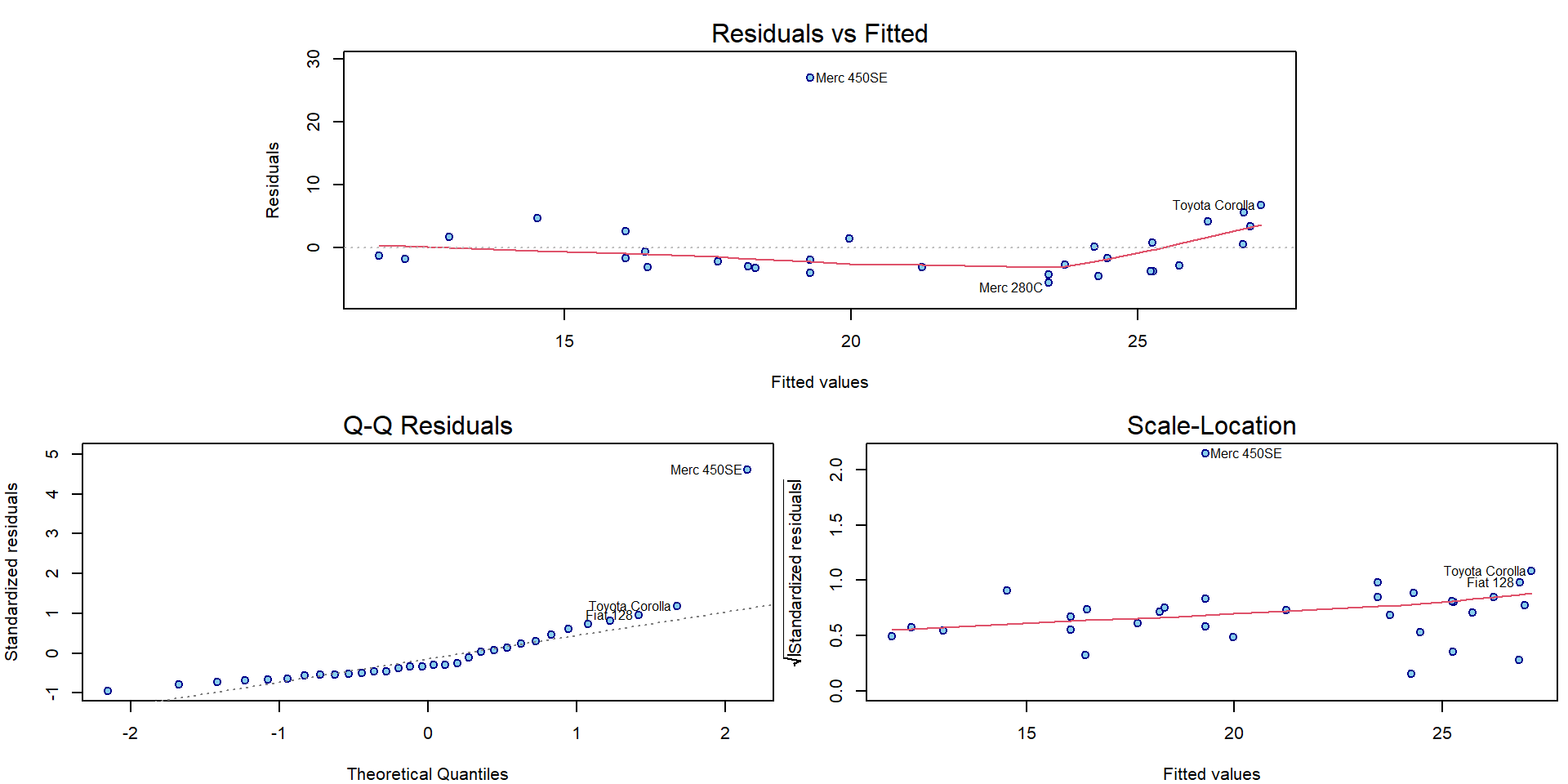
par(mar = c(4,4,2.5,0.5))
plotLM(m3)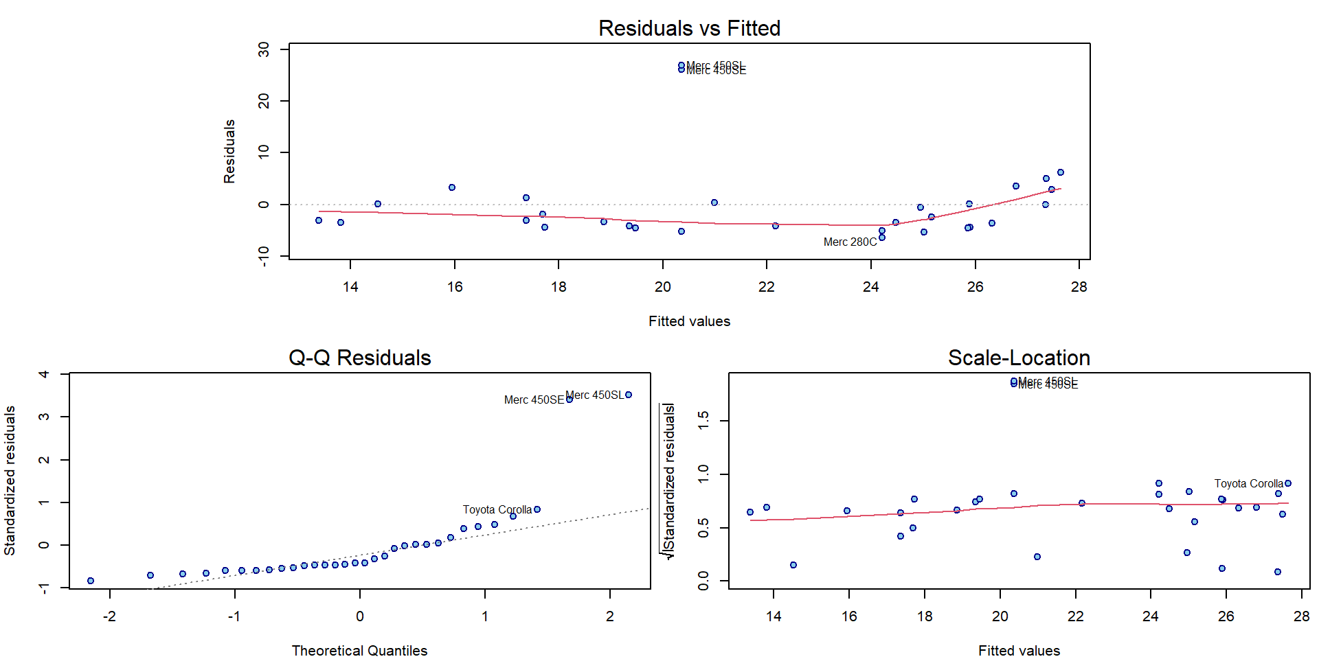
Outlier detection
Consider the outlier model for \(t\)-th observation: \[ \mathtt{m[t]}: \quad \mathbf{Y} | \mathbb{X} \sim \mathsf{N}_n \left(\mathbb{X} \boldsymbol{\beta} + \gamma_t e_{t}, \sigma^2\right) \] where \(\gamma_t\) corresponds to the correction for mis-specified expected value for \(t\)-th observation. The test for the null hypothesis \(\gamma_t = 0\) can, thus, be interpreted as a test of outlyingness. Computing the estimates and p-values by fitting each model is expensive:
detect_out <- sapply(1:nrow(mtcars_out2), function(t){
  e_t <- rep(0, nrow(mtcars_out2))
  e_t[t] <- 1
  m_t <- lm(mpg ~ disp + e_t, data = mtcars_out2)
  sm_t <- summary(m_t)
  c(gamma = coef(m_t)[3], pval = sm_t$coefficients[3,4])
})
detect_out <- as.matrix(t(detect_out))
rownames(detect_out) <- rownames(mtcars_out2)
detect_out
## gamma.e_t pval
## Mazda RX4 -3.63031996 6.562469e-01
## Mazda RX4 Wag -3.63031996 6.562469e-01
## Datsun 710 -3.76319359 6.481609e-01
## Hornet 4 Drive 0.41740501 9.590654e-01
## Hornet Sportabout 1.42269199 8.634978e-01
## Valiant -4.20050769 6.043703e-01
## Duster 360 -3.28998150 6.906123e-01
## Merc 240D -0.57799107 9.437276e-01
## Merc 230 -2.48066158 7.620177e-01
## Merc 280 -5.21528957 5.213017e-01
## Merc 280C -6.67304174 4.107839e-01
## Merc 450SE 26.99502683 1.939898e-04
## Merc 450SL 27.92816956 9.792204e-05
## Merc 450SLC -5.35392142 5.092974e-01
## Cadillac Fleetwood -3.53427996 6.838905e-01
## Lincoln Continental -3.98224436 6.439643e-01
## Chrysler Imperial 0.19516625 9.817706e-01
## Fiat 128 5.46854240 5.102819e-01
## Honda Civic 3.18599109 7.023010e-01
## Toyota Corolla 6.84209253 4.103355e-01
## Toyota Corona -4.66209538 5.702579e-01
## Dodge Challenger -3.53100773 6.660052e-01
## AMC Javelin -4.34651343 5.939652e-01
## Camaro Z28 -4.71528622 5.667092e-01
## Pontiac Firebird 3.57671457 6.694144e-01
## Fiat X1-9 -0.06203056 9.940632e-01
## Porsche 914-2 0.11717257 9.886483e-01
## Lotus Europa 3.88660530 6.386617e-01
## Ford Pantera L -2.01574876 8.070219e-01
## Ferrari Dino -5.57187302 4.946092e-01
## Maserati Bora -4.66233306 5.671040e-01
## Volvo 142E -4.73213141 5.643603e-01From lecture we know that the estimates can be obtained as \(\widehat{\gamma}_t = U_t / m_{tt}\) where \(U_t\) are residuals from the model with all observations:
deleted_residual <- residuals(m3)/(1-hatvalues(m3))
all.equal(detect_out[,1], deleted_residual)
## [1] TRUEwhich is often called a deleted residual. Then, an estimate for the variance is \[ \widehat{\mathsf{var}} \left[\widehat{\gamma}_t | \mathbb{X}\right] = \widehat{\frac{\sigma^2}{m_{tt}}} = \frac{1}{m_{tt}} \mathsf{MS}_{e,t}^{out} = \frac{1}{m_{tt}} \mathsf{MS}_{e} \dfrac{n-r-(U_t^{std})^2}{n-r-1} \] which is used to obtain p-values:
vars <- 1/(1-hatvalues(m3)) * sum(residuals(m3)^2)/m3$df.residual * (m3$df.residual-stdres(m3)^2)/(m3$df.residual - 1)
tstats <- deleted_residual / sqrt(vars)
pvals <- 2 * pt(abs(tstats), df=m3$df.residual-1, lower.tail = FALSE)
all.equal(detect_out[,2], pvals)
## [1] TRUEHowever, we are facing multiple testing problem, hence, p-values should be adjusted by e.g. Bonferroni correction (multiply p-value by number of tests, cut if exceeds 1):
(pval_bonf <- pmin(1, pvals * length(pvals)))## [1] 1.000000000 1.000000000 1.000000000 1.000000000 1.000000000 1.000000000 1.000000000 1.000000000
## [9] 1.000000000 1.000000000 1.000000000 0.006207674 0.003133505 1.000000000 1.000000000 1.000000000
## [17] 1.000000000 1.000000000 1.000000000 1.000000000 1.000000000 1.000000000 1.000000000 1.000000000
## [25] 1.000000000 1.000000000 1.000000000 1.000000000 1.000000000 1.000000000 1.000000000 1.000000000NEVER exclude observations in an automatic manner! It depends on the underlying model, which may not be suitable. Exclude observations only under reasonable justification:
- Is it data error?
- Is the assumed model correct?
- Can we explain the unusual observation?
- Are we interested in capturing this anomally?
2. Leverage points
Unlike the outlying observations, the leverage points are atypical with respect to the domain of the covariate - the \(x\) axis. Similarly as before, we will introduce some leverage points in the dataset and we will investigate the effect on the final model.
mtcars_lev1 <- mtcars
i3 <- 1 # try also 20
mtcars_lev1$disp[i3] <- 0

summary(m4 <- lm(mpg ~ disp , data = mtcars_lev1))
##
## Call:
## lm(formula = mpg ~ disp, data = mtcars_lev1)
##
## Residuals:
## Min 1Q Median 3Q Max
## -7.614 -2.135 -0.872 2.079 7.971
##
## Coefficients:
## Estimate Std. Error t value Pr(>|t|)
## (Intercept) 28.613789 1.275205 22.439 < 2e-16 ***
## disp -0.037760 0.004915 -7.682 1.44e-08 ***
## ---
## Signif. codes: 0 '***' 0.001 '**' 0.01 '*' 0.05 '.' 0.1 ' ' 1
##
## Residual standard error: 3.557 on 30 degrees of freedom
## Multiple R-squared: 0.663, Adjusted R-squared: 0.6518
## F-statistic: 59.02 on 1 and 30 DF, p-value: 1.435e-08Visually:
par(mfrow = c(1,1), mar = c(4,4,0.5,0.5))
plot(mpg ~ disp, data = mtcars_lev1,
     xlab = expression(Displacement~"["~inch^3~"]"), ylab = "Miles per Gallon",
     pch = 22, bg = "lightblue", col = "navyblue")

points(mtcars$mpg[i3] ~ mtcars$disp[i3], pch = 22, bg = "lightblue", col="navyblue", cex = 2)
arrows(x0 = mtcars$disp[i3], x1 = mtcars_lev1$disp[i3], y0 = mtcars$mpg[i3])
points(mtcars_lev1$mpg[i3] ~ mtcars_lev1$disp[i3], pch = 22, bg = "red", cex = 2)
abline(m1, col = "blue", lwd = 2)
abline(m4, col = "red", lwd = 2)
And, again, the second leverage point can make the whole situation even worse:
mtcars_lev2 <- mtcars_lev1
i4 <- 25 # try also 15
mtcars_lev2$disp[i4] <- mtcars_lev2$disp[i4] + 300

summary(m5 <- lm(mpg ~ disp , data = mtcars_lev2))
##
## Call:
## lm(formula = mpg ~ disp, data = mtcars_lev2)
##
## Residuals:
## Min 1Q Median 3Q Max
## -5.676 -2.926 -1.731 1.990 12.132
##
## Coefficients:
## Estimate Std. Error t value Pr(>|t|)
## (Intercept) 26.67608 1.42921 18.665 < 2e-16 ***
## disp -0.02801 0.00513 -5.461 6.34e-06 ***
## ---
## Signif. codes: 0 '***' 0.001 '**' 0.01 '*' 0.05 '.' 0.1 ' ' 1
##
## Residual standard error: 4.339 on 30 degrees of freedom
## Multiple R-squared: 0.4985, Adjusted R-squared: 0.4818
## F-statistic: 29.82 on 1 and 30 DF, p-value: 6.345e-06is <- c(i3, i4)
par(mfrow = c(1,1), mar = c(4,4,0.5,0.5))
plot(mpg ~ disp, data = mtcars_lev2,
xlab = expression(Displacement~"["~inch^3~"]"), ylab = "Miles per Gallon",
pch = 22, bg = "lightblue", col = "navyblue")
points(mtcars$mpg[is] ~ mtcars$disp[is], pch = 22, bg = "lightblue", col="navyblue", cex = 2)
arrows(x0 = mtcars$disp[is], x1 = mtcars_lev2$disp[is], y0 = mtcars$mpg[is])
points(mtcars_lev2$mpg[is] ~ mtcars_lev2$disp[is], pch = 22, bg = "red", cex = 2)
abline(m1, col = "blue", lwd = 2)
abline(m4, col = "red", lwd = 2)
abline(m5, col = "red4", lwd = 2)
Note, that both leverage points are tied with response values close
to the mean. They are only atypical with respect to the displacement
value. However, according to the model, these response values are
atypical for such extreme disp values and, hence, could be
considered outliers as well.
par(mar = c(4,4,2.5,0.5))
plotLM(m5)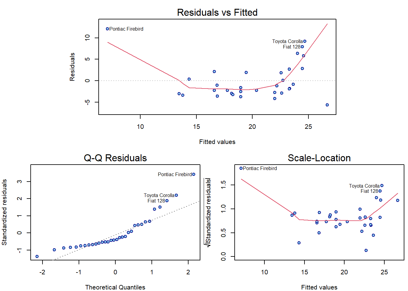
Individual work
- Compare the estimated parameters for all three models and investigate the effect of the introduced leverage points.
- Note, that the leverage points do not have that much effect (compared to the outlying observations) if they are supposed to be only atypical with respect to the covariate domain (and not with respect to the response).
Leverage point detection
The diagonal element \(h_{tt} = \mathbf{x}_t^\top \left(\mathbb{X}^\top\mathbb{X}\right)^{-1} \mathbf{x}_t\) of hat matrix \(\mathbb{H} = \mathbb{X} \left(\mathbb{X}^\top\mathbb{X}\right)^{-1} \mathbb{X}^\top\) is called t-th leverage. In model with intercept the model can be rewritten with centered regressors, which yields \[ h_{tt} = \frac{1}{n} + (x_{t1} - \overline{x}_{1}, \ldots, x_{tp} - \overline{x}_{p}) \; \mathbb{Q} \; (x_{t1} - \overline{x}_{1}, \ldots, x_{tp} - \overline{x}_{p})^\top \] where \(\mathbb{Q} = \left(\widetilde{\mathbb{X}}^\top \widetilde{\mathbb{X}}\right)^{-1}\) and \(\widetilde{\mathbb{X}} = \left(\mathbf{X}_1-\overline{x}_1 \;|\; \cdots \;|\; \mathbf{X}_p-\overline{x}_p \right)\). We immediately see that \(h_{tt}\) expresses how distant the \(t\)-th observation is from the centers \(\overline{x}_{j}\). Moreover, it is obvious that the response values do not play any role here.
Remember that \[ \mathsf{var} \left[U_i | \mathbb{X}\right] = \mathsf{var} \left[Y_i - \widehat{Y}_i | \mathbb{X}\right] = \sigma^2 m_{ii} = \sigma^2 ( 1 - h_{ii}) \] so the residuals have lower variance with higher leverages. Thus, fitted values of high leverage observations are forced to be closer to the observed response values than those of low leverage observations.
cbind(1:nrow(mtcars), hatvalues(m1), hatvalues(m4), hatvalues(m5))## [,1] [,2] [,3] [,4]
## Mazda RX4 1 0.04175345 0.12855487 0.10851146
## Mazda RX4 Wag 2 0.04175345 0.03949911 0.03913339
## Datsun 710 3 0.06287776 0.05771681 0.05383078
## Hornet 4 Drive 4 0.03281262 0.03323977 0.03198326
## Hornet Sportabout 5 0.06634737 0.06568482 0.05305800
## Valiant 6 0.03131875 0.03125100 0.03139251
## Duster 360 7 0.06634737 0.06568482 0.05305800
## Merc 240D 8 0.04607550 0.04317565 0.04217303
## Merc 230 9 0.04823068 0.04502293 0.04367979
## Merc 280 10 0.03961728 0.03770159 0.03761849
## Merc 280C 11 0.03961728 0.03770159 0.03761849
## Merc 450SE 12 0.03551733 0.03603943 0.03356593
## Merc 450SL 13 0.03551733 0.03603943 0.03356593
## Merc 450SLC 14 0.03551733 0.03603943 0.03356593
## Cadillac Fleetwood 15 0.15350324 0.14708477 0.10970322
## Lincoln Continental 16 0.14164508 0.13607159 0.10195663
## Chrysler Imperial 17 0.12322550 0.11893856 0.08994030
## Fiat 128 18 0.07978295 0.07253109 0.06544206
## Honda Civic 19 0.08171734 0.07423297 0.06676639
## Toyota Corolla 20 0.08475684 0.07690929 0.06884589
## Toyota Corona 21 0.05694842 0.05255566 0.04973593
## Dodge Challenger 22 0.04724688 0.04751241 0.04085751
## AMC Javelin 23 0.04252647 0.04295222 0.03788662
## Camaro Z28 24 0.06112763 0.06074692 0.04970580
## Pontiac Firebird 25 0.09142639 0.08925601 0.33338018
## Fiat X1-9 26 0.07959158 0.07236279 0.06531102
## Porsche 914-2 27 0.05685559 0.05247505 0.04967168
## Lotus Europa 28 0.06987638 0.06383510 0.05864718
## Ford Pantera L 29 0.06163070 0.06122352 0.05002844
## Ferrari Dino 30 0.04668149 0.04369428 0.04259720
## Maserati Bora 31 0.04162205 0.04207243 0.03732129
## Volvo 142E 32 0.05653197 0.05219412 0.04944771A rule of thumb for leverage detection:
which(hatvalues(m5) > 3 * m5$rank / nrow(mtcars_lev2))## Pontiac Firebird
## 25Individual work
- Consider a situation, where both types of atypical observations are introduced in the model - the leverage points and, also, the outlying observations.
- How much bad can the model become with bad leverage points and bad outlying observations?
3. Cook’s distance and other influence measures
In general, ?influence.measures provides many other
measures on finding influential observations.
infm <- influence.measures(m5)
head(infm$infmat)
## dfb.1_ dfb.disp dffit cov.r cook.d hat
## Mazda RX4 -0.49125792 0.41452737 -0.49125792 1.051690 0.116839848 0.10851146
## Mazda RX4 Wag -0.04788201 0.02503946 -0.05578819 1.107892 0.001605591 0.03913339
## Datsun 710 -0.04519989 0.03064154 -0.04731038 1.127977 0.001156158 0.05383078
## Hornet 4 Drive 0.03300576 0.01241034 0.08196261 1.090172 0.003450567 0.03198326
## Hornet Sportabout -0.01506783 0.07481180 0.11669108 1.111411 0.006984644 0.05305800
## Valiant -0.05608125 0.00637970 -0.09468729 1.084058 0.004593604 0.03139251apply(infm$is.inf, 2, which)## dfb.1_ dfb.disp dffit cov.r cook.d hat
## 25 25 25 25 25 25We will only show enough to understand the two default plots for linear models:
par(mfrow = c(1,2), mar = c(4,4,2,1.5))
plot(m5, which = 4:5)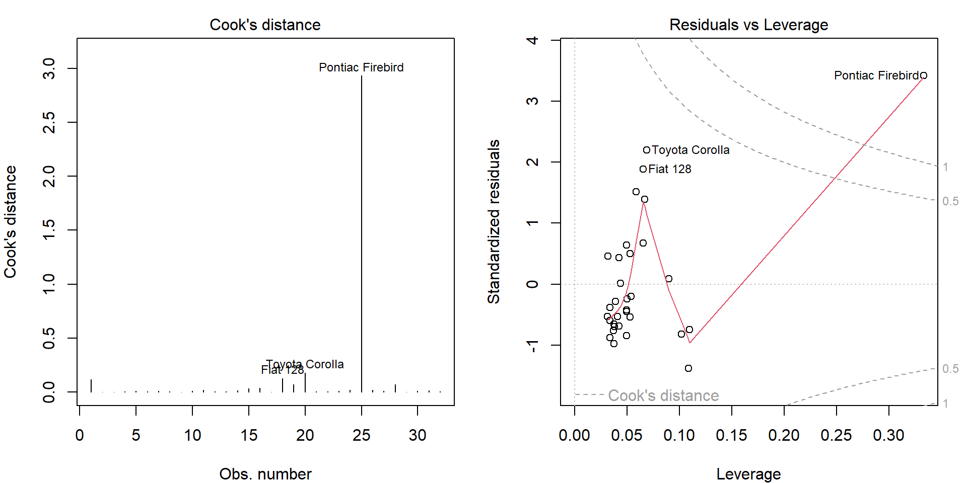
- Standardized residuals: \(U_i^{std} = U_i / \sqrt{\mathsf{MS}_e m_{ii}}\) have zero mean and unit variance.
- Leverages: \(h_{tt}\) measure the irregularity in regression space.
- Cook’s distance: \(D_t = \frac{1}{r \mathsf{MS}_e} \|\widehat{\mathbf{Y}} - \widehat{\mathbf{Y}}_{(-t\bullet)}\|^2 = \frac{1}{r} \frac{h_{tt}}{m_{tt}} \left(U_t^{std}\right)^2\) measures the difference in fitted values estimated by excluding \(t\)-th observation (up to the scale).
Notice that the top 3 observations in Cook’s distance are the
labelled observations in plot.lm() plots.
Given a distance \(d \in \mathbb{R}\) we can express standardized residuals as two functions of \(d\) and leverage \(h\): \(u_{1,2}(h,d) = \pm\sqrt{rd\frac{1-h}{h}}\), which are the dashed grey lines on the right hand side.
Real data example - Animals
We will explore data on animals containing information about the body weight (in kg) and brain weight (in g). See how widely spread the values are:
data(Animals, package = "MASS")
head(Animals)
## body brain
## Mountain beaver 1.35 8.1
## Cow 465.00 423.0
## Grey wolf 36.33 119.5
## Goat 27.66 115.0
## Guinea pig 1.04 5.5
## Dipliodocus 11700.00 50.0summary(Animals)## body brain
## Min. : 0.023 Min. : 0.40
## 1st Qu.: 3.100 1st Qu.: 22.23
## Median : 53.830 Median : 137.00
## Mean : 4278.439 Mean : 574.52
## 3rd Qu.: 479.000 3rd Qu.: 420.00
## Max. :87000.000 Max. :5712.00Hence, original scale is not suitable for modelling purposes. However, on log-scale we observe nice linear trend:
Animals <- transform(Animals, lbody = log2(body), lbrain = log(brain))
par(mfrow = c(1,2), mar = c(4,4,2.5,0.5))
plot(brain ~ body, Animals, main = "Original scale")
plot(lbrain ~ lbody, Animals, main = "Log-scale", bg = "grey80", pch = 21)
abline(mall <- lm(lbrain ~ lbody, data = Animals), col = "red")
dinosaurs <- c("Brachiosaurus", "Dipliodocus", "Triceratops")
arrows(x0 = Animals[dinosaurs, "lbody"], y0 = fitted(mall)[dinosaurs], y1 = Animals[dinosaurs, "lbrain"],
col = "grey30", lty = 2, length = 0.1)
text(lbrain ~ lbody, data = Animals, labels = rownames(Animals), cex = 0.7)
text(2.5, 1, pos = 4, cex = 0.8,
labels = eval(substitute(expression(paste(hat(E), "[ln Y|X=x]", dot(" = "),
be0, " + ", be1, " ", log[2], " x", sep = "")),
list(be0 = format(coef(mall)[1], digits = 3),
be1 = format(coef(mall)[2], digits = 3)))))
text(2.5, 0.1, pos = 4, cex = 0.8,
labels = eval(substitute(expression(paste(hat(E), "[Y|X=2x] / ", hat(E), "[Y|X=x] = ",
exp(hat(beta)[1]), dot(" = "), eb1 , sep = "")),
list(eb1 = format(exp(coef(mall)[2]), digits = 3)))))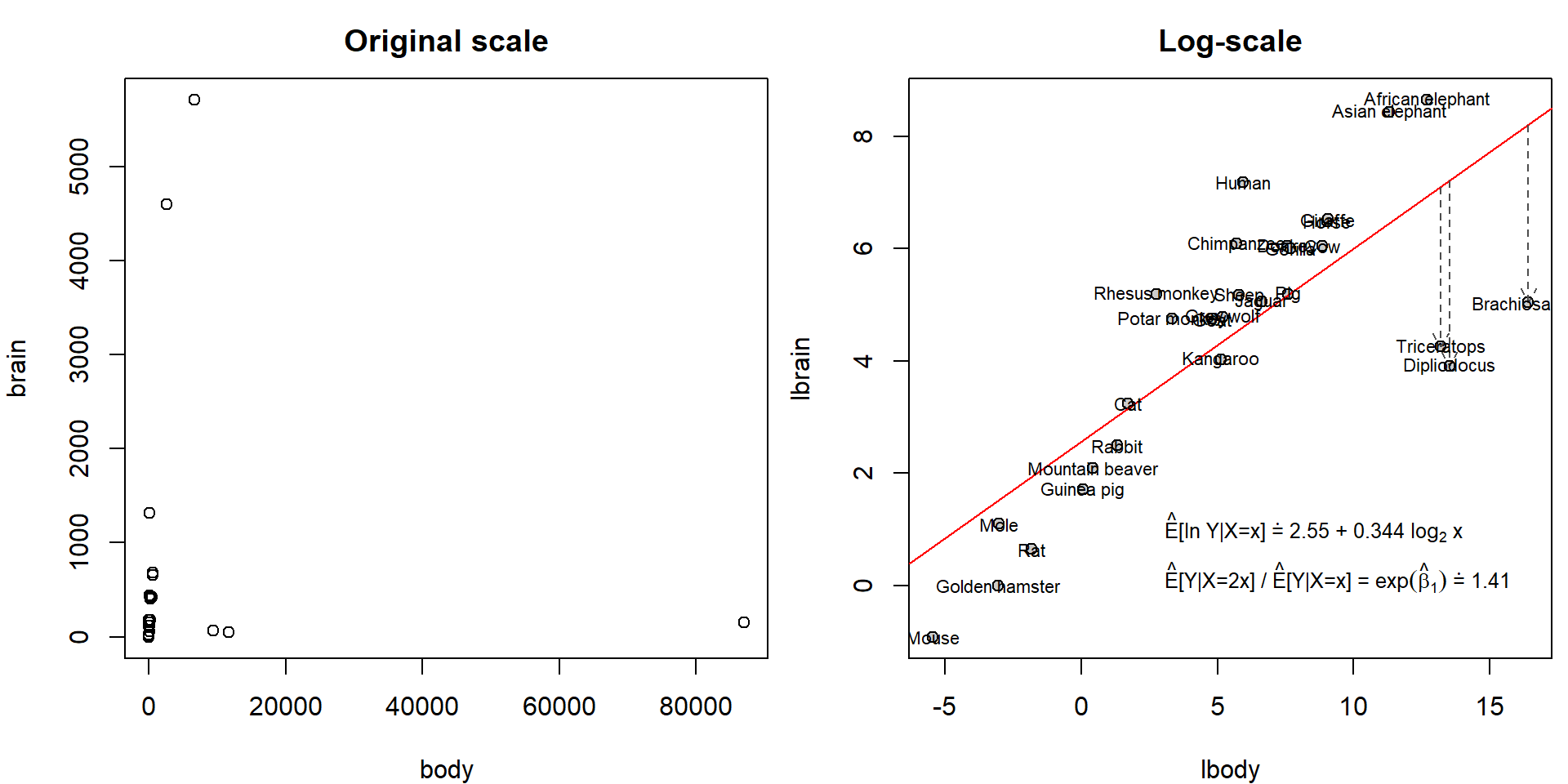 However, it seems that the fitted line is heavily influenced by three
observations: Brachiosaurus, Dipliodocus and Triceratops. Unlike other
observations, these three “animals” are extinct for millions of years.
These exemplars didn’t have the same amount of time to evolve their
brain wrt body. They also didn’t stand the test of time and natural
selection.
However, it seems that the fitted line is heavily influenced by three
observations: Brachiosaurus, Dipliodocus and Triceratops. Unlike other
observations, these three “animals” are extinct for millions of years.
These exemplars didn’t have the same amount of time to evolve their
brain wrt body. They also didn’t stand the test of time and natural
selection.
Before we decide to exclude them, let’s explore the corresponding influential measures:
par(mfrow = c(1,2), mar = c(4,4,2,1.5))
plot(mall, which = 4:5)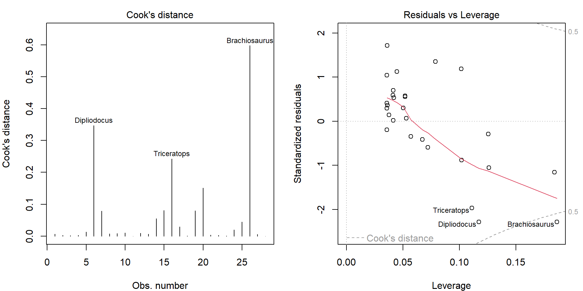
Clearly, these three observations dominate in Cook’s distance. Top 6 observations in terms of deleted residuals:
deleted_residuals <- residuals(mall)/(1-hatvalues(mall))
head(sort(abs(deleted_residuals), decreasing = TRUE))
## Brachiosaurus Dipliodocus Triceratops Human Asian elephant Mouse
## 3.878416 3.726060 3.199214 2.680052 2.160058 1.960872Top 6 observations in terms of hat values:
head(sort(hatvalues(mall), decreasing = TRUE))## Brachiosaurus Mouse Golden hamster Mole Dipliodocus Triceratops
## 0.1862707 0.1839511 0.1261343 0.1256276 0.1172906 0.1110340Let’s compare the difference in the estimated line after exclusion of dinosaurs:
exclude <- c("Brachiosaurus", "Dipliodocus", "Triceratops")
keep <- setdiff(rownames(Animals), exclude)
subAnimals <- Animals[keep,]
msub <- lm(lbrain ~ lbody, data = subAnimals)

par(mfrow = c(1,1), mar = c(4,4,0.5,0.5))
plot(lbrain ~ lbody, data = subAnimals, pch = 21, col = "darkblue", bg = "lightblue",
     xlim = range(Animals$lbody),
     xlab = expression(Log[2](body)~"["~log[2]~"(kg)]"), ylab = "Ln(brain) [ln(g)]")
abline(msub, col = "red", lwd = 2)
text(3, 1.5, pos = 4,
     labels = eval(substitute(expression(paste(hat(E), "[ln Y|X=x]", dot(" = "),
                                               be0, " + ", be1, " ", log[2], " x", sep = "")),
                              list(be0 = format(coef(msub)[1], digits = 3),
                                   be1 = format(coef(msub)[2], digits = 3)))))
text(3, 0.8, pos = 4,
     labels = eval(substitute(expression(paste(hat(E), "[Y|X=2x] / ", hat(E), "[Y|X=x] = ",
                                               exp(hat(beta)[1]), dot(" = "), eb1 , sep = "")),
                              list(eb1 = format(exp(coef(msub)[2]), digits = 3)))))
points(lbrain ~ lbody, data = Animals[exclude,], pch = 25, col = "black", bg = "darkviolet")
text(lbrain ~ lbody, data = Animals[exclude,], labels = exclude, pos = 2)
top3res <- order(abs(residuals(msub)), decreasing = TRUE)[1:3]
text(lbrain ~ lbody, data = subAnimals[top3res,], labels = rownames(subAnimals)[top3res], pos = 2)
legend("bottomright", legend = "Excluded observations", bty = "n",
       pch = 25, pt.bg = "darkviolet")
How do the diagnostic plots look like now?
par(mfrow = c(2,2), mar = c(4,4,2,1.5))
plot(msub, which = c(1:3,5))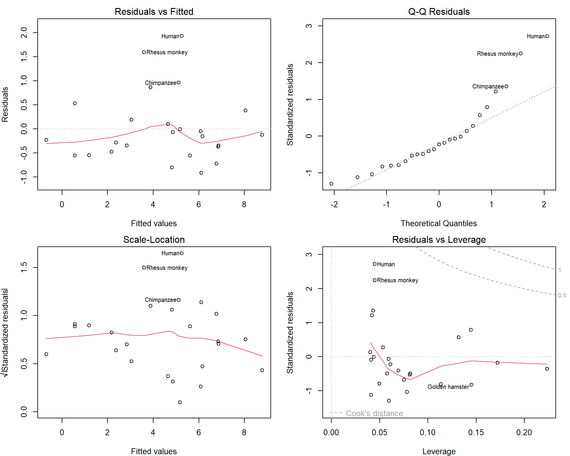
Maybe we should consider excluding Human as well… But this depends on the purpose of our model.