Multiple regression model - additive models

Download this R markdown as: R, Rmd.

Outline of the lab session

Multiple regression model with categorical covariate of multiple levels
Additive model - combination of numeric and categorical covariates
Model selection strategies

Loading the data and libraries

The dataset mtcars (available under the standard R installation) will be used for the purposes of this lab session. Some insight about the data can be taken from the help session (command ?mtcars) or from some outputs provided below.

library(colorspace)
head(mtcars)

##                    mpg cyl disp  hp drat    wt  qsec vs am gear carb
## Mazda RX4         21.0   6  160 110 3.90 2.620 16.46  0  1    4    4
## Mazda RX4 Wag     21.0   6  160 110 3.90 2.875 17.02  0  1    4    4
## Datsun 710        22.8   4  108  93 3.85 2.320 18.61  1  1    4    1
## Hornet 4 Drive    21.4   6  258 110 3.08 3.215 19.44  1  0    3    1
## Hornet Sportabout 18.7   8  360 175 3.15 3.440 17.02  0  0    3    2
## Valiant           18.1   6  225 105 2.76 3.460 20.22  1  0    3    1

str(mtcars)

## 'data.frame':    32 obs. of  11 variables:
##  $ mpg : num  21 21 22.8 21.4 18.7 18.1 14.3 24.4 22.8 19.2 ...
##  $ cyl : num  6 6 4 6 8 6 8 4 4 6 ...
##  $ disp: num  160 160 108 258 360 ...
##  $ hp  : num  110 110 93 110 175 105 245 62 95 123 ...
##  $ drat: num  3.9 3.9 3.85 3.08 3.15 2.76 3.21 3.69 3.92 3.92 ...
##  $ wt  : num  2.62 2.88 2.32 3.21 3.44 ...
##  $ qsec: num  16.5 17 18.6 19.4 17 ...
##  $ vs  : num  0 0 1 1 0 1 0 1 1 1 ...
##  $ am  : num  1 1 1 0 0 0 0 0 0 0 ...
##  $ gear: num  4 4 4 3 3 3 3 4 4 4 ...
##  $ carb: num  4 4 1 1 2 1 4 2 2 4 ...

summary(mtcars)

##       mpg            cyl            disp             hp             drat            wt            qsec     
##  Min.   :10.4   Min.   :4.00   Min.   : 71.1   Min.   : 52.0   Min.   :2.76   Min.   :1.51   Min.   :14.5  
##  1st Qu.:15.4   1st Qu.:4.00   1st Qu.:120.8   1st Qu.: 96.5   1st Qu.:3.08   1st Qu.:2.58   1st Qu.:16.9  
##  Median :19.2   Median :6.00   Median :196.3   Median :123.0   Median :3.69   Median :3.33   Median :17.7  
##  Mean   :20.1   Mean   :6.19   Mean   :230.7   Mean   :146.7   Mean   :3.60   Mean   :3.22   Mean   :17.8  
##  3rd Qu.:22.8   3rd Qu.:8.00   3rd Qu.:326.0   3rd Qu.:180.0   3rd Qu.:3.92   3rd Qu.:3.61   3rd Qu.:18.9  
##  Max.   :33.9   Max.   :8.00   Max.   :472.0   Max.   :335.0   Max.   :4.93   Max.   :5.42   Max.   :22.9  
##        vs              am             gear           carb     
##  Min.   :0.000   Min.   :0.000   Min.   :3.00   Min.   :1.00  
##  1st Qu.:0.000   1st Qu.:0.000   1st Qu.:3.00   1st Qu.:2.00  
##  Median :0.000   Median :0.000   Median :4.00   Median :2.00  
##  Mean   :0.438   Mean   :0.406   Mean   :3.69   Mean   :2.81  
##  3rd Qu.:1.000   3rd Qu.:1.000   3rd Qu.:4.00   3rd Qu.:4.00  
##  Max.   :1.000   Max.   :1.000   Max.   :5.00   Max.   :8.00

Categorical predictor variable

Finally, we will consider a regression dependence of a continuous variable \(Y\) on some categorical covariate \(X\) (taking more than 2 levels). We will consider the number of cylinders (there are four, six, and eight cylinder cars in the data set). Note, that the categorical covariate can be either assumed to be nominal or, also, ordinal.

par(mfrow = c(1,1), mar = c(4,4,0.5,0.5))
boxplot(mpg ~ cyl, data = mtcars, col = "lightblue")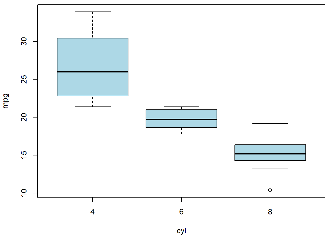

Compare and explain the following models:

fit1 <- lm(mpg ~ cyl, data = mtcars)
summary(fit1)

## 
## Call:
## lm(formula = mpg ~ cyl, data = mtcars)
## 
## Residuals:
##    Min     1Q Median     3Q    Max 
## -4.981 -2.119  0.222  1.072  7.519 
## 
## Coefficients:
##             Estimate Std. Error t value Pr(>|t|)    
## (Intercept)   37.885      2.074   18.27  < 2e-16 ***
## cyl           -2.876      0.322   -8.92  6.1e-10 ***
## ---
## Signif. codes:  0 '***' 0.001 '**' 0.01 '*' 0.05 '.' 0.1 ' ' 1
## 
## Residual standard error: 3.21 on 30 degrees of freedom
## Multiple R-squared:  0.726,  Adjusted R-squared:  0.717 
## F-statistic: 79.6 on 1 and 30 DF,  p-value: 6.11e-10

fit2 <- lm(mpg ~ as.factor(cyl), data = mtcars)
summary(fit2)

## 
## Call:
## lm(formula = mpg ~ as.factor(cyl), data = mtcars)
## 
## Residuals:
##    Min     1Q Median     3Q    Max 
## -5.264 -1.836  0.029  1.389  7.236 
## 
## Coefficients:
##                 Estimate Std. Error t value Pr(>|t|)    
## (Intercept)       26.664      0.972   27.44  < 2e-16 ***
## as.factor(cyl)6   -6.921      1.558   -4.44  0.00012 ***
## as.factor(cyl)8  -11.564      1.299   -8.90  8.6e-10 ***
## ---
## Signif. codes:  0 '***' 0.001 '**' 0.01 '*' 0.05 '.' 0.1 ' ' 1
## 
## Residual standard error: 3.22 on 29 degrees of freedom
## Multiple R-squared:  0.732,  Adjusted R-squared:  0.714 
## F-statistic: 39.7 on 2 and 29 DF,  p-value: 4.98e-09

fit3 <- lm(mpg ~ cyl + I(cyl^2), data = mtcars)
summary(fit3)

## 
## Call:
## lm(formula = mpg ~ cyl + I(cyl^2), data = mtcars)
## 
## Residuals:
##    Min     1Q Median     3Q    Max 
## -5.264 -1.836  0.029  1.389  7.236 
## 
## Coefficients:
##             Estimate Std. Error t value Pr(>|t|)    
## (Intercept)   47.339     11.647    4.06  0.00034 ***
## cyl           -6.308      4.172   -1.51  0.14140    
## I(cyl^2)       0.285      0.345    0.83  0.41607    
## ---
## Signif. codes:  0 '***' 0.001 '**' 0.01 '*' 0.05 '.' 0.1 ' ' 1
## 
## Residual standard error: 3.22 on 29 degrees of freedom
## Multiple R-squared:  0.732,  Adjusted R-squared:  0.714 
## F-statistic: 39.7 on 2 and 29 DF,  p-value: 4.98e-09

Individual work

What are other possible parametrizations that can be used?
Compare the following model with the model denoted as fit2.

mtcars$dummy1 <- as.numeric(mtcars$cyl == 4)
mtcars$dummy1[mtcars$cyl == 8] <- -1

mtcars$dummy2 <- as.numeric(mtcars$cyl == 6)
mtcars$dummy2[mtcars$cyl == 8] <- -1

fit4 <- lm(mpg ~ dummy1 + dummy2, data = mtcars)
summary(fit4)

## 
## Call:
## lm(formula = mpg ~ dummy1 + dummy2, data = mtcars)
## 
## Residuals:
##    Min     1Q Median     3Q    Max 
## -5.264 -1.836  0.029  1.389  7.236 
## 
## Coefficients:
##             Estimate Std. Error t value Pr(>|t|)    
## (Intercept)   20.502      0.594   34.54  < 2e-16 ***
## dummy1         6.161      0.817    7.54  2.6e-08 ***
## dummy2        -0.759      0.920   -0.83     0.42    
## ---
## Signif. codes:  0 '***' 0.001 '**' 0.01 '*' 0.05 '.' 0.1 ' ' 1
## 
## Residual standard error: 3.22 on 29 degrees of freedom
## Multiple R-squared:  0.732,  Adjusted R-squared:  0.714 
## F-statistic: 39.7 on 2 and 29 DF,  p-value: 4.98e-09

Can you reconstruct model fit2 from the model above (fit4)? Look at the output of the summary() function and explain the statistical tests that are provided for each column of the summary table (in model fit2 and model fit4).
Think of some other parametrization that could be suitable and try to implement them in the R software.

Categorical and numeric covariate as regressors

What happens when we add the weight of the car wt into the formula of model fit2?

mtcars$fcyl <- factor(mtcars$cyl)

fit5 <- lm(mpg ~ fcyl + wt, data = mtcars)
summary(fit5)

## 
## Call:
## lm(formula = mpg ~ fcyl + wt, data = mtcars)
## 
## Residuals:
##    Min     1Q Median     3Q    Max 
## -4.589 -1.236 -0.516  1.384  5.792 
## 
## Coefficients:
##             Estimate Std. Error t value Pr(>|t|)    
## (Intercept)   33.991      1.888   18.01  < 2e-16 ***
## fcyl6         -4.256      1.386   -3.07  0.00472 ** 
## fcyl8         -6.071      1.652   -3.67  0.00100 ***
## wt            -3.206      0.754   -4.25  0.00021 ***
## ---
## Signif. codes:  0 '***' 0.001 '**' 0.01 '*' 0.05 '.' 0.1 ' ' 1
## 
## Residual standard error: 2.56 on 28 degrees of freedom
## Multiple R-squared:  0.837,  Adjusted R-squared:  0.82 
## F-statistic: 48.1 on 3 and 28 DF,  p-value: 3.59e-11

The model has 4 coefficients: \[ \mathsf{E} \left[Y | F = f, X = x \right] = \beta_1 + \beta_2 \mathbb{1} [f = 6] + \beta_3 \mathbb{1} [f = 8] + \beta_4 x \] with the following interpretation: \[ \begin{aligned} \beta_1 &= \mathsf{E} \left[Y | F = 4, X = 0 \right], \\ \beta_2 &= \mathsf{E} \left[Y | F = 6, X = x \right] - \mathsf{E} \left[Y | F = 4, X = x \right], \\ \beta_3 &= \mathsf{E} \left[Y | F = 8, X = x \right] - \mathsf{E} \left[Y | F = 4, X = x \right], \\ \beta_4 &= \mathsf{E} \left[Y | F = f, X = x+1 \right] - \mathsf{E} \left[Y | F = f, X = x \right]. \end{aligned} \]

Especially, the difference between two levels of the factor variable is always the same regardless of the value \(x\). Similarly, the linear trend has the same slope regardless of the factor \(f\). Hence, the resulting fit are 3 parallel lines - one for each factor group:

PCH <- c(21, 22, 24)
DARK <- rainbow_hcl(3, c = 80, l = 35)
COL <- rainbow_hcl(3, c = 80, l = 50)
BGC <- rainbow_hcl(3, c = 80, l = 70)
names(PCH) <- names(COL) <- names(BGC) <- levels(mtcars$fcyl)

par(mfrow = c(1,1), mar = c(4,4,0.5,0.5))
plot(mpg ~ wt, data = mtcars, 
     ylab = "Miles per gallon", 
     xlab = "Weight [1000 lbs]",
     pch = PCH[fcyl], col = COL[fcyl], bg = BGC[fcyl])
abline(a = coef(fit5)[1], b = coef(fit5)[4],
       col = COL[1], lwd = 2)
abline(a = coef(fit5)[1]+coef(fit5)[2], b = coef(fit5)[4],
       col = COL[2], lwd = 2)
abline(a = coef(fit5)[1]+coef(fit5)[3], b = coef(fit5)[4],
       col = COL[3], lwd = 2)
legend("topright", legend = levels(mtcars$fcyl), bty = "n",
       col = COL, pt.bg = BGC, pch = PCH, lty = 1, lwd = 2)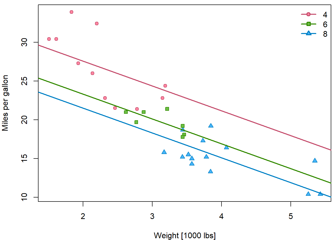

Individual work

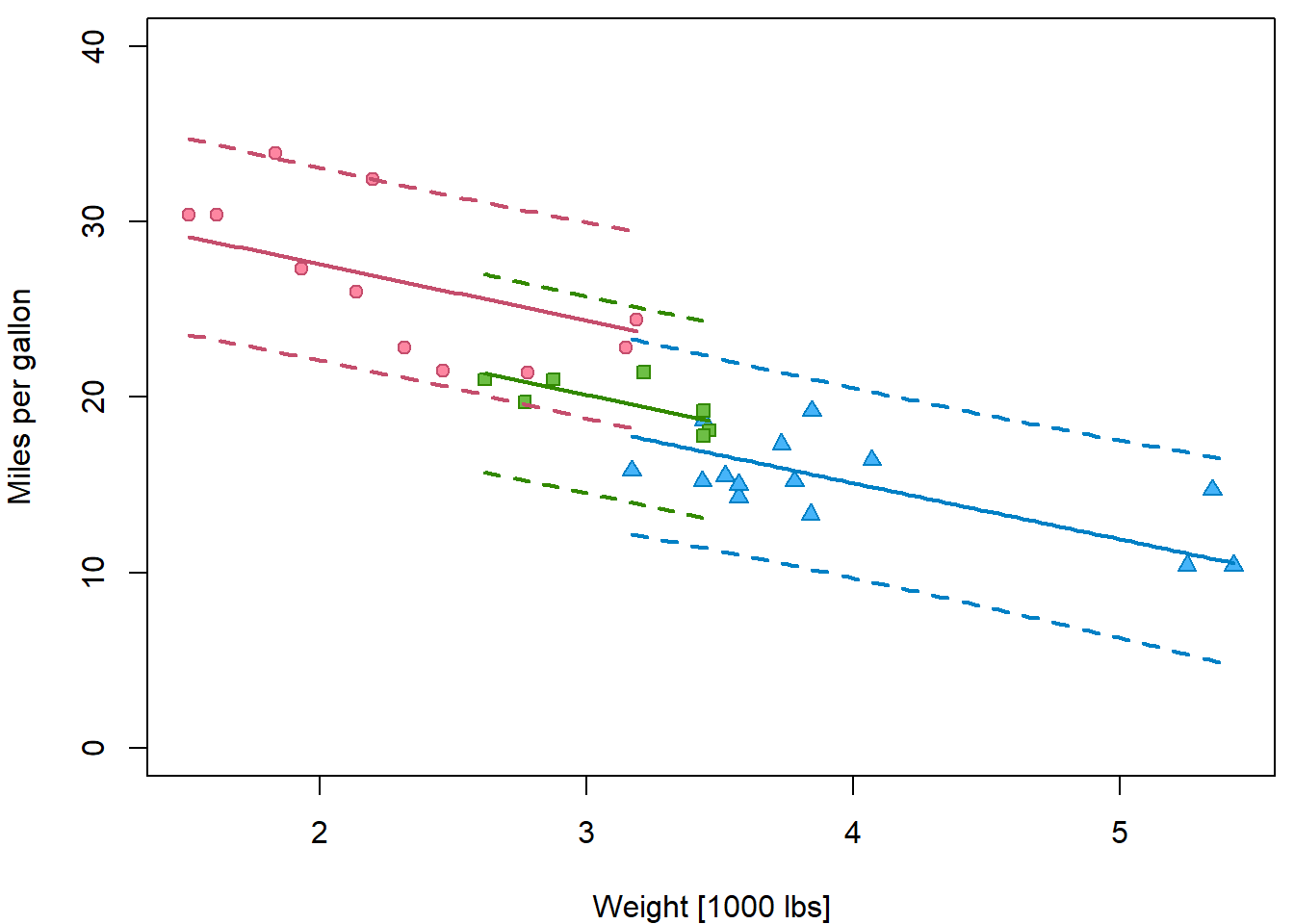
Insert prediction intervals into the previous plot by following these steps:

Compute range of wt for each level of fcyl.
Create newdata for each fcyl level separately with a grid of wt values in the range specific for this cylinder count.
Use predict on fit5 three times for these 3 new datasets with option interval="prediction".
Instead of abline for plotting the estimated line use lines on the point estimate fit to plot it only on a relevant range.
Insert lines for lower and upper bounds, choose appropriate colors and different line type lty and width lwd.

ranges <- tapply(mtcars$wt, mtcars$fcyl, range)

par(mfrow = c(1,1), mar = c(4,4,0.5,0.5))
plot(mpg ~ wt, data = mtcars, 
     ylab = "Miles per gallon", 
     xlab = "Weight [1000 lbs]",
     ylim = c(0,40),
     pch = PCH[fcyl], col = COL[fcyl], bg = BGC[fcyl])
for(l in levels(mtcars$fcyl)){
  xgrid <- seq(ranges[[l]][1], ranges[[l]][2], length.out = 101)
  newdata <- data.frame(fcyl = l, 
                        wt = xgrid)
  pred <- predict(fit5, newdata = newdata, interval = "prediction")
  lines(x = xgrid, y = pred[,"fit"], col = COL[l], lwd = 2)
  lines(x = xgrid, y = pred[,"lwr"], col = COL[l], lwd = 2, lty = 2)
  lines(x = xgrid, y = pred[,"upr"], col = COL[l], lwd = 2, lty = 2)
}

Additive model

Let us consider a model that tries to explain miles per gallon mpg of a vehicle by: disp, hp and drat as in previous exercise.

For simplicity, we now consider linear parametrizations and categorical covariates that only require single column in the model matrix. The following model (as well as all the models above) is additive. The effect of one covariate does not depend on the values of other covariates: \[ \beta_k = \mathsf{E} \left[Y | X_k = x_k + 1, \mathbf{X}_{-k} = \mathbf{x}_{-k}\right] - \left[Y | \mathbf{X} = \mathbf{x} \right] \]

fit_add <- lm(mpg ~ disp + hp + drat, data = mtcars)
summary(fit_add)

## 
## Call:
## lm(formula = mpg ~ disp + hp + drat, data = mtcars)
## 
## Residuals:
##    Min     1Q Median     3Q    Max 
## -5.122 -1.845 -0.446  1.134  6.496 
## 
## Coefficients:
##             Estimate Std. Error t value Pr(>|t|)   
## (Intercept) 19.34429    6.37088    3.04   0.0051 **
## disp        -0.01923    0.00937   -2.05   0.0496 * 
## hp          -0.03123    0.01334   -2.34   0.0266 * 
## drat         2.71498    1.48737    1.83   0.0786 . 
## ---
## Signif. codes:  0 '***' 0.001 '**' 0.01 '*' 0.05 '.' 0.1 ' ' 1
## 
## Residual standard error: 3.01 on 28 degrees of freedom
## Multiple R-squared:  0.775,  Adjusted R-squared:  0.751 
## F-statistic: 32.2 on 3 and 28 DF,  p-value: 3.28e-09

Which regressors seem to have significant effect? Which of them seem irrelevant?

Model selection strategies

Considering the critical level of \(\alpha = 0.05\), we can not reject the null hypothesis \(H_0; \beta_4 = 0\), which (in words) means that the consumption of the car is independent of the rear axle ratio. Thus, instead of the model with 3 predictor variables we can consider a smaller (restricted) model with the remaining 2 covariates.

fit_add2 <- lm(mpg ~ disp + hp, data = mtcars)
(sumfit_add2 <- summary(fit_add2))

## 
## Call:
## lm(formula = mpg ~ disp + hp, data = mtcars)
## 
## Residuals:
##    Min     1Q Median     3Q    Max 
## -4.795 -2.304 -0.825  1.858  6.936 
## 
## Coefficients:
##             Estimate Std. Error t value Pr(>|t|)    
## (Intercept)  30.7359     1.3316   23.08  < 2e-16 ***
## disp         -0.0303     0.0074   -4.10  0.00031 ***
## hp           -0.0248     0.0134   -1.86  0.07368 .  
## ---
## Signif. codes:  0 '***' 0.001 '**' 0.01 '*' 0.05 '.' 0.1 ' ' 1
## 
## Residual standard error: 3.13 on 29 degrees of freedom
## Multiple R-squared:  0.748,  Adjusted R-squared:  0.731 
## F-statistic: 43.1 on 2 and 29 DF,  p-value: 2.06e-09

In the restricted model, using again the critical value of \(\alpha = 0.05\), we can again see that the null hypothesis \(H_0: \beta_2 = 0\) is not rejected – the corresponding \(p\)-value \(0.07368\) is slightly higher than \(0.05\). Thus, we can again consider a submodel, where the car consumption is only explained by the information about the engine displacement:

fit_add3 <- lm(mpg ~ disp, data = mtcars)
summary(fit_add3)

## 
## Call:
## lm(formula = mpg ~ disp, data = mtcars)
## 
## Residuals:
##    Min     1Q Median     3Q    Max 
## -4.892 -2.202 -0.963  1.627  7.231 
## 
## Coefficients:
##             Estimate Std. Error t value Pr(>|t|)    
## (Intercept) 29.59985    1.22972   24.07  < 2e-16 ***
## disp        -0.04122    0.00471   -8.75  9.4e-10 ***
## ---
## Signif. codes:  0 '***' 0.001 '**' 0.01 '*' 0.05 '.' 0.1 ' ' 1
## 
## Residual standard error: 3.25 on 30 degrees of freedom
## Multiple R-squared:  0.718,  Adjusted R-squared:  0.709 
## F-statistic: 76.5 on 1 and 30 DF,  p-value: 9.38e-10

In the model above, both statistical tests return significant \(p\)-value and the model can not be further reduced. Thus, we performed the model selection procedure. From all considered models we selected one final model that is (in some well-defined sense) the most appropriate one. This particular selection strategy is called the stepwise backward selection strategy.

Stepwise backward selection

The idea is to fit a full model firstly and, consecutively, to reduce the model by taking out the less significant predictors. The final model is the one in which no other predictor can be added. This is the procedure that we just applied above.

Stepwise forward selection

The idea is reverse. We start with all possible (three in this case) simple regression models (as we fitted them above) and we conclude that the most significant dependence is for the model with the dependence of the consumption on the displacement – compare the \(p\)-values below:

summary(fit_disp <- lm(mpg ~ disp, data = mtcars))

## 
## Call:
## lm(formula = mpg ~ disp, data = mtcars)
## 
## Residuals:
##    Min     1Q Median     3Q    Max 
## -4.892 -2.202 -0.963  1.627  7.231 
## 
## Coefficients:
##             Estimate Std. Error t value Pr(>|t|)    
## (Intercept) 29.59985    1.22972   24.07  < 2e-16 ***
## disp        -0.04122    0.00471   -8.75  9.4e-10 ***
## ---
## Signif. codes:  0 '***' 0.001 '**' 0.01 '*' 0.05 '.' 0.1 ' ' 1
## 
## Residual standard error: 3.25 on 30 degrees of freedom
## Multiple R-squared:  0.718,  Adjusted R-squared:  0.709 
## F-statistic: 76.5 on 1 and 30 DF,  p-value: 9.38e-10

summary(fit_hp <- lm(mpg ~ hp, data = mtcars))

## 
## Call:
## lm(formula = mpg ~ hp, data = mtcars)
## 
## Residuals:
##    Min     1Q Median     3Q    Max 
## -5.712 -2.112 -0.885  1.582  8.236 
## 
## Coefficients:
##             Estimate Std. Error t value Pr(>|t|)    
## (Intercept)  30.0989     1.6339   18.42  < 2e-16 ***
## hp           -0.0682     0.0101   -6.74  1.8e-07 ***
## ---
## Signif. codes:  0 '***' 0.001 '**' 0.01 '*' 0.05 '.' 0.1 ' ' 1
## 
## Residual standard error: 3.86 on 30 degrees of freedom
## Multiple R-squared:  0.602,  Adjusted R-squared:  0.589 
## F-statistic: 45.5 on 1 and 30 DF,  p-value: 1.79e-07

summary(fit_drat <- lm(mpg ~ drat, data = mtcars))

## 
## Call:
## lm(formula = mpg ~ drat, data = mtcars)
## 
## Residuals:
##    Min     1Q Median     3Q    Max 
##  -9.08  -2.68  -0.21   2.30   9.02 
## 
## Coefficients:
##             Estimate Std. Error t value Pr(>|t|)    
## (Intercept)    -7.52       5.48   -1.37     0.18    
## drat            7.68       1.51    5.10  1.8e-05 ***
## ---
## Signif. codes:  0 '***' 0.001 '**' 0.01 '*' 0.05 '.' 0.1 ' ' 1
## 
## Residual standard error: 4.49 on 30 degrees of freedom
## Multiple R-squared:  0.464,  Adjusted R-squared:  0.446 
## F-statistic:   26 on 1 and 30 DF,  p-value: 1.78e-05

Thus, the model that we use to proceed further is the model where the consumption is explained by the displacement. In the second step of the stepwise forward selection procedure we look for another covariate (out of two remaining ones, hp, or drat) which can be added into the model (meaning that the corresponding \(p\)-value of the test is significant). We consider two models:

fit_for1 <- lm(mpg ~ disp + hp, data = mtcars)
summary(fit_for1)

## 
## Call:
## lm(formula = mpg ~ disp + hp, data = mtcars)
## 
## Residuals:
##    Min     1Q Median     3Q    Max 
## -4.795 -2.304 -0.825  1.858  6.936 
## 
## Coefficients:
##             Estimate Std. Error t value Pr(>|t|)    
## (Intercept)  30.7359     1.3316   23.08  < 2e-16 ***
## disp         -0.0303     0.0074   -4.10  0.00031 ***
## hp           -0.0248     0.0134   -1.86  0.07368 .  
## ---
## Signif. codes:  0 '***' 0.001 '**' 0.01 '*' 0.05 '.' 0.1 ' ' 1
## 
## Residual standard error: 3.13 on 29 degrees of freedom
## Multiple R-squared:  0.748,  Adjusted R-squared:  0.731 
## F-statistic: 43.1 on 2 and 29 DF,  p-value: 2.06e-09

fit_for2 <- lm(mpg ~ disp + drat, data = mtcars)
summary(fit_for2)

## 
## Call:
## lm(formula = mpg ~ disp + drat, data = mtcars)
## 
## Residuals:
##    Min     1Q Median     3Q    Max 
## -5.127 -2.205 -0.583  1.450  6.988 
## 
## Coefficients:
##             Estimate Std. Error t value Pr(>|t|)    
## (Intercept) 21.84488    6.74797    3.24    0.003 ** 
## disp        -0.03569    0.00665   -5.37  9.2e-06 ***
## drat         1.80203    1.54209    1.17    0.252    
## ---
## Signif. codes:  0 '***' 0.001 '**' 0.01 '*' 0.05 '.' 0.1 ' ' 1
## 
## Residual standard error: 3.23 on 29 degrees of freedom
## Multiple R-squared:  0.731,  Adjusted R-squared:  0.712 
## F-statistic: 39.4 on 2 and 29 DF,  p-value: 5.39e-09

In both cases we observe the \(p\)-value for the added covariate which is larger than \(0.05\). Thus, the final model is the model denoted as fit_add3 or fit_disp, where only disp is included.

Individual work

Note, that both model selection strategies (backward and forward) returned the same final model. This is, however, not always the case.
Discuss some obvious advantages and disadvantages of both selection strategies.
What would happen if you also consider other covariates such as wt, cyl, am, vs, \(\ldots\)?

cor(mtcars[,1:11])

##          mpg     cyl    disp      hp     drat      wt    qsec      vs       am    gear     carb
## mpg   1.0000 -0.8522 -0.8476 -0.7762  0.68117 -0.8677  0.4187  0.6640  0.59983  0.4803 -0.55093
## cyl  -0.8522  1.0000  0.9020  0.8324 -0.69994  0.7825 -0.5912 -0.8108 -0.52261 -0.4927  0.52699
## disp -0.8476  0.9020  1.0000  0.7909 -0.71021  0.8880 -0.4337 -0.7104 -0.59123 -0.5556  0.39498
## hp   -0.7762  0.8324  0.7909  1.0000 -0.44876  0.6587 -0.7082 -0.7231 -0.24320 -0.1257  0.74981
## drat  0.6812 -0.6999 -0.7102 -0.4488  1.00000 -0.7124  0.0912  0.4403  0.71271  0.6996 -0.09079
## wt   -0.8677  0.7825  0.8880  0.6587 -0.71244  1.0000 -0.1747 -0.5549 -0.69250 -0.5833  0.42761
## qsec  0.4187 -0.5912 -0.4337 -0.7082  0.09120 -0.1747  1.0000  0.7445 -0.22986 -0.2127 -0.65625
## vs    0.6640 -0.8108 -0.7104 -0.7231  0.44028 -0.5549  0.7445  1.0000  0.16835  0.2060 -0.56961
## am    0.5998 -0.5226 -0.5912 -0.2432  0.71271 -0.6925 -0.2299  0.1683  1.00000  0.7941  0.05753
## gear  0.4803 -0.4927 -0.5556 -0.1257  0.69961 -0.5833 -0.2127  0.2060  0.79406  1.0000  0.27407
## carb -0.5509  0.5270  0.3950  0.7498 -0.09079  0.4276 -0.6562 -0.5696  0.05753  0.2741  1.00000

Model selection criteria

There are also other selection strategies based on various selection criteria. Typically used criteria are, for instance, the Akaike’s Information Criterion (AIC) or Bayesian Information Criterion (BIC). But there are also others.

For the AIC criterion, there is a standard R function AIC():

AIC(fit_add3)

## [1] 170.2

### compare also with the AIC for the remaining two (simple) regression models
AIC(fit_hp)

## [1] 181.2

AIC(fit_drat)

## [1] 190.8

The BIC criterion is implemented, for instance, in the library flexmix (installation with the command install.packages("flexmix") is needed)

library(flexmix)
BIC(fit_add3)

## [1] 174.6

AIC(fit_add3, k=log(nobs(fit_add3))) # the same

## [1] 174.6

### compare also with the BIC for the remaining two (simple) regression models
BIC(fit_hp)

## [1] 185.6

BIC(fit_drat)

## [1] 195.2

Individual work

Consider both, AIC and BIC criterion and use them to perform the model selection approach. The smaller the value the better the fit.
Use some literature or references and find out how AIC and BIC are calculated.
What are some discussed advantages/disadvantages of all four model selection approaches?

Multiple regression model - additive models

Jan Vávra

Exercise 5

Outline of the lab session

Loading the data and libraries

Categorical predictor variable

Individual work

Categorical and numeric covariate as regressors

Individual work

Additive model

Model selection strategies

Stepwise backward selection

Stepwise forward selection

Individual work

Model selection criteria

Individual work