Interactions, transformations, hierarchy
Jan Vávra
Exercise 6
Download this R markdown as: R, Rmd.
Outline of the lab session
- Multiple regression model with interactions
- Transformations of the explanatory variables
- Hierarchically well formulated model vs. non-hierarchical model
Loading the data and libraries
For the purpose of this lab session we will consider the dataset
Dris from the R library mffSM. We will be
interested in the dependence of the yield on the amount of magnesium
concentration (yield ~ Mg) and the amount of the calcium
concentration (yield ~ Ca).
library("mffSM")
library("colorspace")
data(Dris, package = "mffSM")
All together, there are 368 observations available in the dataset and 6 different measurements (although, we will not use all of them). A brief insight about the data can be taken from the following code:
dim(Dris)## [1] 368 6head(Dris)## yield N P K Ca Mg
## 1 5.47 470 47 320 47 11
## 2 5.63 530 48 357 60 16
## 3 5.63 530 48 310 63 16
## 4 4.84 482 47 357 47 13
## 5 4.84 506 48 294 52 15
## 6 4.21 500 45 283 61 14summary(Dris)## yield N P K Ca Mg
## Min. :1.920 Min. :268.0 Min. :32.00 Min. :200.0 Min. :29.00 Min. : 8.00
## 1st Qu.:4.040 1st Qu.:427.0 1st Qu.:43.00 1st Qu.:338.0 1st Qu.:41.75 1st Qu.:10.00
## Median :4.840 Median :473.0 Median :49.00 Median :377.0 Median :49.00 Median :11.00
## Mean :4.864 Mean :469.9 Mean :48.65 Mean :375.4 Mean :51.45 Mean :11.64
## 3rd Qu.:5.558 3rd Qu.:518.0 3rd Qu.:54.00 3rd Qu.:407.0 3rd Qu.:59.00 3rd Qu.:13.00
## Max. :8.792 Max. :657.0 Max. :72.00 Max. :580.0 Max. :95.00 Max. :22.00Firstly, we visualize marginal dependence of yield on the magnesium concentration and the calcium concentration.
par(mfrow = c(1,2), mar = c(4,4,0.5,0.5))
plot(yield ~ Mg, data = Dris, pch = 22, bg = "gray",
     xlab = "Magnesium concentration", ylab = "Yield")
plot(yield ~ Ca, data = Dris, pch = 22, bg = "gray",
     xlab = "Calcium concentration", ylab = "Yield")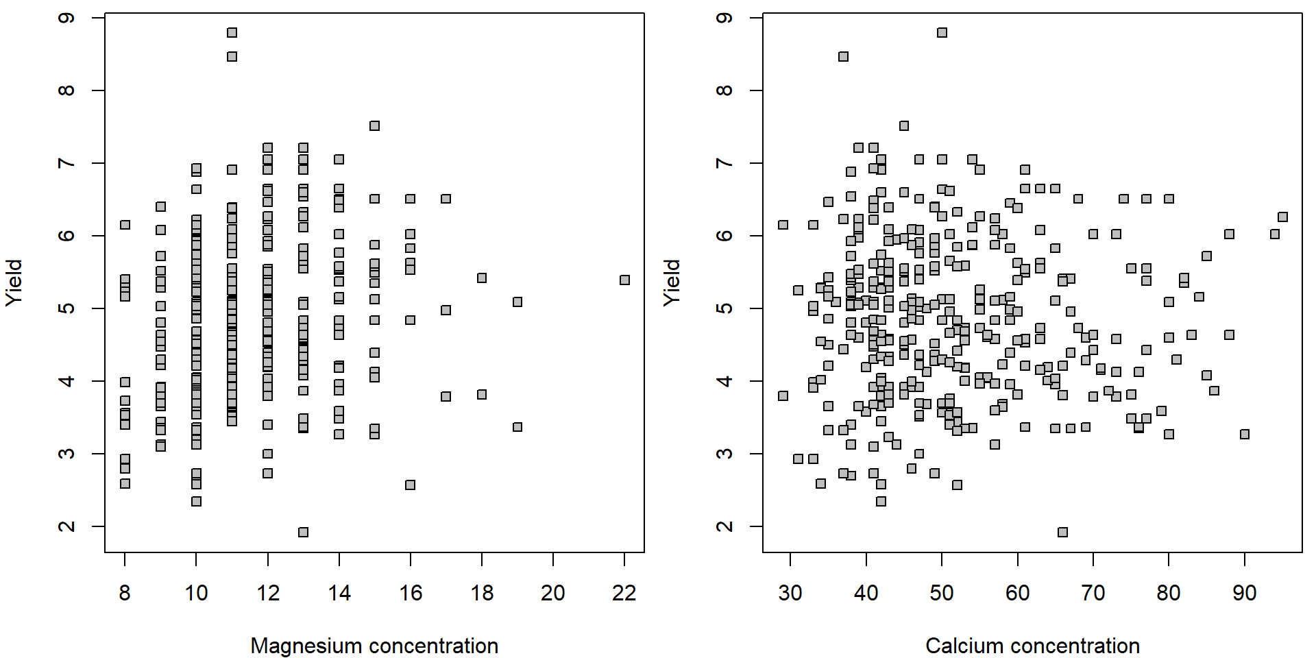
Note, that the points are not equally distributed along the \(x\) axis. There are way more points at the left corners of the scatterplots than in the right parts. This suggests that a logarithmic transformation (of the magnesium and calcium concentration) could help to align the data more uniformly along the \(x\) axis,
For more intuitive interpretation we use the logarithm with the base
two (meaning that unit increase of the logaritmically transformed
covariates, i.e.,
\(\log_2(x) + 1 = \log_2 (x) \cdot \log_2 2 =
\log_2 (2 x)\) equals double amount of the original
covariate).
Dris <- transform(Dris,
                  lMg = log2(Mg), lMg2 = (log2(Mg))^2,
                  lCa = log2(Ca), lCa2 = (log2(Ca))^2,
                  lN = log2(N), lN2=(log2(N))^2)
The same scatterplots but x-axis in on logarithmic scale.
par(mfrow = c(1,2), mar = c(4,4,0.5,0.5))
plot(yield ~ lMg, data = Dris, pch = 22, bg = "gray",
xlab = "Magnesium concentration [log scale]", ylab = "Yield")
plot(yield ~ lCa, data = Dris, pch = 22, bg = "gray",
xlab = "Calcium concentration [log scale]", ylab = "Yield")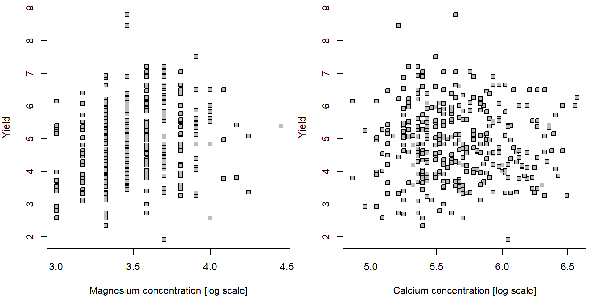 Plotting functions in R also provide an option to turn an axis to the
log scale. It does not offer you the option to choose the base but
adjusts x-axis to keep the labels of original values. Now the labels on
the x-axis are not equidistant:
Plotting functions in R also provide an option to turn an axis to the
log scale. It does not offer you the option to choose the base but
adjusts x-axis to keep the labels of original values. Now the labels on
the x-axis are not equidistant:
par(mfrow = c(1,2), mar = c(4,4,0.5,0.5))
plot(yield ~ Mg, data = Dris, pch = 22, bg = "gray", log = "x",
     xlab = "Magnesium concentration", ylab = "Yield")
plot(yield ~ Ca, data = Dris, pch = 22, bg = "gray", log = "x",
     xlab = "Calcium concentration", ylab = "Yield")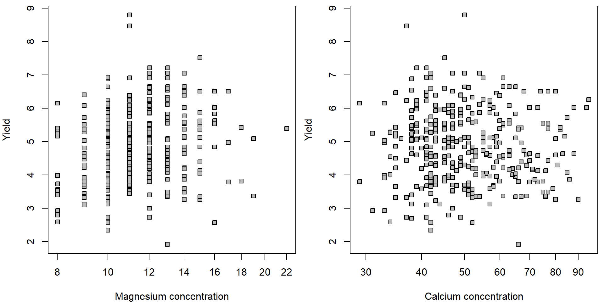
For the following, we will use the transformed data.
Individual work
- Visualize the marginal distributions of the original and the transformed variables. Comment on the skewness of the distribution.
- Use the techniques from previous exercises to reason the log-trend compared to the linear trend.
- For the log-transformed covariates suppress the x-axis labels
(
xaxt = "n") and add your own labels with original scale withaxis().
1. Simple and multiple linear regression models
Let us start with two simple regression models (one explanatory variable only) and we compare these models with a multiple regression model (with both explanatory variables being used at the same time).
summary(m10 <- lm(yield ~ lMg, data = Dris))##
## Call:
## lm(formula = yield ~ lMg, data = Dris)
##
## Residuals:
## Min 1Q Median 3Q Max
## -3.1194 -0.7412 -0.0741 0.7451 3.9841
##
## Coefficients:
## Estimate Std. Error t value Pr(>|t|)
## (Intercept) 1.4851 0.7790 1.907 0.0574 .
## lMg 0.9605 0.2208 4.349 1.77e-05 ***
## ---
## Signif. codes: 0 '***' 0.001 '**' 0.01 '*' 0.05 '.' 0.1 ' ' 1
##
## Residual standard error: 1.07 on 366 degrees of freedom
## Multiple R-squared: 0.04915, Adjusted R-squared: 0.04655
## F-statistic: 18.92 on 1 and 366 DF, p-value: 1.772e-05summary(m01 <- lm(yield ~ lCa, data = Dris))##
## Call:
## lm(formula = yield ~ lCa, data = Dris)
##
## Residuals:
## Min 1Q Median 3Q Max
## -2.9021 -0.8094 -0.0388 0.7211 3.9279
##
## Coefficients:
## Estimate Std. Error t value Pr(>|t|)
## (Intercept) 5.4561 0.9119 5.983 5.22e-09 ***
## lCa -0.1049 0.1614 -0.650 0.516
## ---
## Signif. codes: 0 '***' 0.001 '**' 0.01 '*' 0.05 '.' 0.1 ' ' 1
##
## Residual standard error: 1.096 on 366 degrees of freedom
## Multiple R-squared: 0.001153, Adjusted R-squared: -0.001576
## F-statistic: 0.4227 on 1 and 366 DF, p-value: 0.516Both marginal models can be now compared with a larger model, containing both predictor variables additively:
summary(m11 <- lm(yield ~ lMg + lCa, data = Dris))##
## Call:
## lm(formula = yield ~ lMg + lCa, data = Dris)
##
## Residuals:
## Min 1Q Median 3Q Max
## -2.9514 -0.7210 -0.0838 0.7700 4.0120
##
## Coefficients:
## Estimate Std. Error t value Pr(>|t|)
## (Intercept) 3.4026 0.9525 3.572 0.000402 ***
## lMg 1.3998 0.2531 5.530 6.11e-08 ***
## lCa -0.6140 0.1805 -3.402 0.000742 ***
## ---
## Signif. codes: 0 '***' 0.001 '**' 0.01 '*' 0.05 '.' 0.1 ' ' 1
##
## Residual standard error: 1.055 on 365 degrees of freedom
## Multiple R-squared: 0.07838, Adjusted R-squared: 0.07333
## F-statistic: 15.52 on 2 and 365 DF, p-value: 3.396e-07Note, there are quite different values for the estimated parameters when being interested in the effect of magnesium or the effect of calcium. Which model should be taken as a reference one?
Individual work
Interpret the models fitted above – try to explain the meaning of the estimated parameters. In particular, focus on the following:
- Interpret the estimated regression coefficients in the models.
- What is being tested on the rows started with ‘lMg’ and ‘lCa’?
- When comparing all three models, which one is, according your our opinion, the most suitable one?
Quadratic trend
In the following, we will try slightly more complex (multiple) regression models:
summary(m20 <- lm(yield ~ lMg + lMg2, data = Dris))##
## Call:
## lm(formula = yield ~ lMg + lMg2, data = Dris)
##
## Residuals:
## Min 1Q Median 3Q Max
## -3.1942 -0.7636 -0.0413 0.8089 3.8957
##
## Coefficients:
## Estimate Std. Error t value Pr(>|t|)
## (Intercept) -18.7523 7.6276 -2.458 0.01442 *
## lMg 12.3814 4.2881 2.887 0.00412 **
## lMg2 -1.6030 0.6011 -2.667 0.00800 **
## ---
## Signif. codes: 0 '***' 0.001 '**' 0.01 '*' 0.05 '.' 0.1 ' ' 1
##
## Residual standard error: 1.061 on 365 degrees of freedom
## Multiple R-squared: 0.06732, Adjusted R-squared: 0.06221
## F-statistic: 13.17 on 2 and 365 DF, p-value: 2.994e-06summary(m02 <- lm(yield ~ lCa + lCa2, data = Dris))##
## Call:
## lm(formula = yield ~ lCa + lCa2, data = Dris)
##
## Residuals:
## Min 1Q Median 3Q Max
## -2.9082 -0.8314 -0.0488 0.6949 3.8889
##
## Coefficients:
## Estimate Std. Error t value Pr(>|t|)
## (Intercept) -4.6108 12.7956 -0.360 0.719
## lCa 3.4343 4.4900 0.765 0.445
## lCa2 -0.3098 0.3928 -0.789 0.431
##
## Residual standard error: 1.097 on 365 degrees of freedom
## Multiple R-squared: 0.002853, Adjusted R-squared: -0.002611
## F-statistic: 0.5222 on 2 and 365 DF, p-value: 0.5937Is there some statistical improvements in the two models above?
And what about the following models?
summary(m21 <- lm(yield ~ lMg + lMg2 + lCa, data = Dris)) ##
## Call:
## lm(formula = yield ~ lMg + lMg2 + lCa, data = Dris)
##
## Residuals:
## Min 1Q Median 3Q Max
## -3.0260 -0.7554 -0.1068 0.7474 3.9233
##
## Coefficients:
## Estimate Std. Error t value Pr(>|t|)
## (Intercept) -16.9375 7.5351 -2.248 0.025186 *
## lMg 12.8838 4.2282 3.047 0.002479 **
## lMg2 -1.6116 0.5923 -2.721 0.006824 **
## lCa -0.6160 0.1789 -3.444 0.000641 ***
## ---
## Signif. codes: 0 '***' 0.001 '**' 0.01 '*' 0.05 '.' 0.1 ' ' 1
##
## Residual standard error: 1.045 on 364 degrees of freedom
## Multiple R-squared: 0.09675, Adjusted R-squared: 0.0893
## F-statistic: 13 on 3 and 364 DF, p-value: 4.408e-08summary(m12 <- lm(yield ~ lMg + lCa + lCa2, data = Dris))##
## Call:
## lm(formula = yield ~ lMg + lCa + lCa2, data = Dris)
##
## Residuals:
## Min 1Q Median 3Q Max
## -2.9605 -0.7377 -0.1027 0.7755 3.9817
##
## Coefficients:
## Estimate Std. Error t value Pr(>|t|)
## (Intercept) -4.3463 12.3118 -0.353 0.724
## lMg 1.3944 0.2535 5.501 7.13e-08 ***
## lCa 2.1151 4.3269 0.489 0.625
## lCa2 -0.2387 0.3782 -0.631 0.528
## ---
## Signif. codes: 0 '***' 0.001 '**' 0.01 '*' 0.05 '.' 0.1 ' ' 1
##
## Residual standard error: 1.055 on 364 degrees of freedom
## Multiple R-squared: 0.07938, Adjusted R-squared: 0.0718
## F-statistic: 10.46 on 3 and 364 DF, p-value: 1.284e-06summary(m22 <- lm(yield ~ lMg + lMg2 + lCa + lCa2, data = Dris)) ##
## Call:
## lm(formula = yield ~ lMg + lMg2 + lCa + lCa2, data = Dris)
##
## Residuals:
## Min 1Q Median 3Q Max
## -3.0262 -0.7583 -0.1083 0.7455 3.9182
##
## Coefficients:
## Estimate Std. Error t value Pr(>|t|)
## (Intercept) -18.26667 13.29798 -1.374 0.17040
## lMg 12.78321 4.31420 2.963 0.00325 **
## lMg2 -1.59767 0.60418 -2.644 0.00854 **
## lCa -0.08582 4.37164 -0.020 0.98435
## lCa2 -0.04638 0.38209 -0.121 0.90345
## ---
## Signif. codes: 0 '***' 0.001 '**' 0.01 '*' 0.05 '.' 0.1 ' ' 1
##
## Residual standard error: 1.047 on 363 degrees of freedom
## Multiple R-squared: 0.09678, Adjusted R-squared: 0.08683
## F-statistic: 9.724 on 4 and 363 DF, p-value: 1.758e-07What is now the effect of the magnesium concentration on the expected (estimated) amount of yield? How this effect can be quantified using different models?
We can actually visualize the effect of the magnesium concentration on the yield (using different models fitted above). Specifically, we are interested in the effect of the change of lMg by additional log2(1.1) which corresponds with the increase of Mg by 10%). What will be the corresponding change of the expected amount of yield, i.e. \(\mathsf{E} [\mathtt{yield} | \mathtt{lMg}, \mathtt{lCa}]\)?
Dris <- transform(Dris, jMg = Mg + runif(nrow(Dris), -0.5, 0.5))
Dris <- transform(Dris, ljMg = log2(jMg))

eps <- 0.1
delta <- log2(1+eps)
lMg.grid <- seq(min(Dris$lMg), max(Dris$lMg)-delta, length = 1000)
effect.lMg <- function(b1,b2) b1*delta + b2*(2*delta*lMg.grid + delta^2)

YLIM <- range(effect.lMg(coef(m20)['lMg'], coef(m20)['lMg2']),
              effect.lMg(coef(m21)['lMg'], coef(m21)['lMg2']),
              effect.lMg(coef(m22)['lMg'], coef(m22)['lMg2']))

par(mfrow = c(1,2), mar = c(4,4,2,0.5))
plot(lMg.grid, effect.lMg(coef(m20)['lMg'], coef(m20)['lMg2']), type="l",
     xlab = "log2(Mg)", ylab = "Change of expected yield",
     main = "The effect of 10%-increase of Mg on the yield",
     col = "blue", lwd = 2, ylim = YLIM)
lines(lMg.grid, effect.lMg(coef(m21)['lMg'], coef(m21)['lMg2']),
      lwd=2, col="red")
lines(lMg.grid, effect.lMg(coef(m22)['lMg'], coef(m22)['lMg2']),
      lwd=2, col="darkgreen", lty="dotted")
abline(h=delta * coef(m10)['lMg'], lwd=2, col="violetred")
abline(h=delta * coef(m11)['lMg'], lwd=2, col="violet")
abline(h=delta * coef(m12)['lMg'], lwd=2, col="saddlebrown", lty="dotted")
abline(h=0, lty="dotted")
legend("topright", legend=c("m20", "m21", "m22", "m10", "m11", "m12"),
       bty="n", ncol=2, lwd=2, cex=1.3,
       col=c("blue", "red", "darkgreen","violetred", "violet", "saddlebrown"),
       lty=c("solid", "solid", "dotted", "solid", "solid", "dotted"))
rug(Dris$ljMg)
## Warning in rug(Dris$ljMg): some values will be clippedMg.grid <- seq(min(Dris$Mg), max(Dris$Mg)-1, length = 1000);
effect.Mg <- function(b1,b2){
return(b1*(log2(Mg.grid+1) - log2(Mg.grid)) +
b2*((log2(1+Mg.grid))^2 - (log2(Mg.grid))^2))
}
YLIM <- range(effect.Mg(coef(m20)['lMg'], coef(m20)['lMg2']),
effect.Mg(coef(m21)['lMg'], coef(m21)['lMg2']),
effect.Mg(coef(m22)['lMg'], coef(m22)['lMg2']))
plot(Mg.grid, effect.Mg(coef(m20)['lMg'], coef(m20)['lMg2']), type="l",
xlab = "Mg", ylab = "Change of expected yield",
main = "The effect of increase of Mg by +1 on the yield",
col = "blue", lwd=2, ylim=YLIM)
lines(Mg.grid, effect.Mg(coef(m21)['lMg'], coef(m21)['lMg2']),
lwd=2, col="red")
lines(Mg.grid, effect.Mg(coef(m22)['lMg'], coef(m22)['lMg2']),
lwd=2, col="darkgreen", lty="dotted")
lines(Mg.grid, coef(m10)['lMg']*(log2(Mg.grid+1) - log2(Mg.grid)),
lwd=2, col="violetred")
lines(Mg.grid, coef(m11)['lMg']*(log2(Mg.grid+1) - log2(Mg.grid)),
lwd=2, col="violet")
lines(Mg.grid, coef(m12)['lMg']*(log2(Mg.grid+1) - log2(Mg.grid)),
lwd=2, col="saddlebrown", lty="dotted")
abline(h=0, lty="dotted")
legend("topright", legend=c("m20", "m21", "m22", "m10", "m11", "m12"),
bty="n", ncol=2, lwd=2, cex=1.3,
col=c("blue", "red", "darkgreen","violetred", "violet", "saddlebrown"),
lty=c("solid", "solid", "dotted", "solid", "solid", "dotted"))
rug(Dris$jMg)## Warning in rug(Dris$jMg): some values will be clipped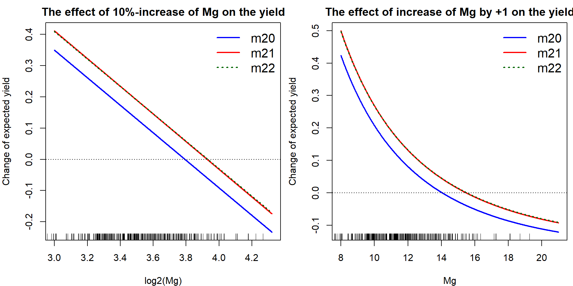
Individual work
- Considering the models above, how would you (statistically) answer a question whether given the information about the magnesium (‘Mg’) the amount of yield is independent of the concentration of the calcium?
- How would you test that given Mg (with the quadratic dependence) the amount of ‘yield’ is independent of Ca?
- Can we say that the amount of yield is independent of Ca?
- Can we say that given Mg and Ca the amount of yield is independent of N?
2. Regression models with simple interactions
The interactions in the model allow for modelling a flexible effect
of some covariate given the value of some other covariate (or multiple
covariates). We consider a simple model with one interaction term
(denoted as lMg:lCa):
summary(m1_inter <- lm(yield ~ lMg + lCa + lMg:lCa, data = Dris))##
## Call:
## lm(formula = yield ~ lMg + lCa + lMg:lCa, data = Dris)
##
## Residuals:
## Min 1Q Median 3Q Max
## -2.9833 -0.7326 -0.1275 0.7797 3.9535
##
## Coefficients:
## Estimate Std. Error t value Pr(>|t|)
## (Intercept) -23.653 11.878 -1.991 0.04719 *
## lMg 9.046 3.356 2.696 0.00735 **
## lCa 4.159 2.096 1.984 0.04802 *
## lMg:lCa -1.346 0.589 -2.285 0.02288 *
## ---
## Signif. codes: 0 '***' 0.001 '**' 0.01 '*' 0.05 '.' 0.1 ' ' 1
##
## Residual standard error: 1.049 on 364 degrees of freedom
## Multiple R-squared: 0.09141, Adjusted R-squared: 0.08392
## F-statistic: 12.21 on 3 and 364 DF, p-value: 1.254e-07- What is the interpretation of the estimated parameters now?
- What is the effect of the magnesium concentration and the calcium concentration on the amount of yield?
- Compare the interaction model above with the model below (multiple model with three explanatory variables, where the last variable \(Z\) is created artificially from the magnesium concentration and the calcium concentration).
Dris$Z <- Dris$lMg * Dris$lCa
summary(m1_Z <- lm(yield ~ lMg + lCa + Z, data = Dris))
##
## Call:
## lm(formula = yield ~ lMg + lCa + Z, data = Dris)
##
## Residuals:
## Min 1Q Median 3Q Max
## -2.9833 -0.7326 -0.1275 0.7797 3.9535
##
## Coefficients:
## Estimate Std. Error t value Pr(>|t|)
## (Intercept) -23.653 11.878 -1.991 0.04719 *
## lMg 9.046 3.356 2.696 0.00735 **
## lCa 4.159 2.096 1.984 0.04802 *
## Z -1.346 0.589 -2.285 0.02288 *
## ---
## Signif. codes: 0 '***' 0.001 '**' 0.01 '*' 0.05 '.' 0.1 ' ' 1
##
## Residual standard error: 1.049 on 364 degrees of freedom
## Multiple R-squared: 0.09141, Adjusted R-squared: 0.08392
## F-statistic: 12.21 on 3 and 364 DF, p-value: 1.254e-07Again, we can quantify the effect of the magnesium concentration on the yield however, this time we have to properly take into account the underlying concentration of calcium. How can be this done?
Mg.grid <- seq(min(Dris$Mg), max(Dris$Mg), length = 5)
blues <- c("lightblue", "skyblue", "deepskyblue", "blue", "navyblue")
Ca.grid <- seq(min(Dris$Ca), max(Dris$Ca), length = 1000)
lCa.grid <- seq(min(Dris$lCa), max(Dris$lCa), length = 1000)
eps <- 0.1;
delta <- log2(1+eps)


par(mfrow = c(1, 2), mar = c(4,4,2,0.5))
plot(lCa.grid,
     delta*coef(m1_inter)['lMg'] + delta*coef(m1_inter)['lMg:lCa'] * lCa.grid,
     xlab = "log2(Ca)", ylab = "Change of expected yield",
     main = "The effect of 10%-increase of Mg on the yield",
     col = "blue", type="l", lwd=2)

plot(Ca.grid,
     coef(m1_inter)['lMg'] * (log2(Mg.grid[3]+1)-log2(Mg.grid[3])) +
     coef(m1_inter)['lMg:lCa'] * (log2(Mg.grid[3]+1)-log2(Mg.grid[3])) * log2(Ca.grid),
     xlab = "Ca", ylab = "Change of expected yield",
     main = "The effect of increase of Mg by +1 on the yield",
     type="n")
for(mg in 1:5){
  lines(Ca.grid,
        coef(m1_inter)['lMg'] * (log2(Mg.grid[mg]+1)-log2(Mg.grid[mg])) +
        coef(m1_inter)['lMg:lCa'] * (log2(Mg.grid[mg]+1)-log2(Mg.grid[mg])) * log2(Ca.grid),
        col = blues[mg], lty=1, lwd=2)
}
legend("topright", paste0("Mg = ", format(Mg.grid, digits = 3)),
       col = blues, lty = 1, lwd = 2)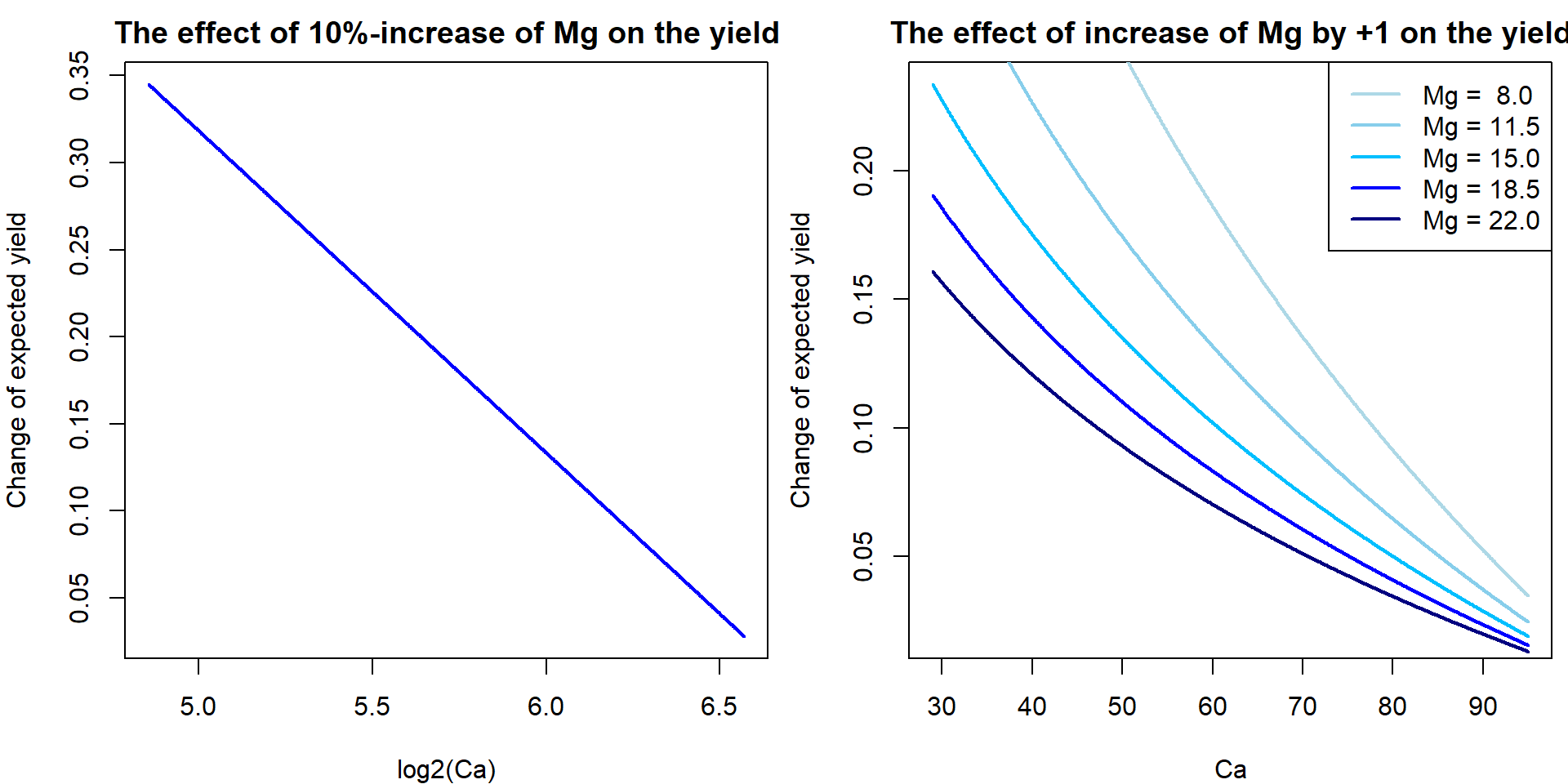
3. Interations with categorical covariates
Let us return to the dataset from Exercise 2:
peat <- read.csv("http://www.karlin.mff.cuni.cz/~vavraj/nmfm334/data/peat.csv",
                 header = TRUE, stringsAsFactors = TRUE)
We have tried to explore the relationship between Nitrogen concentration and depth:
XLAB <- "Depth [cm]"
YLAB <- "Nitrogen concentration [weight %]"
XLIM <- range(peat[, "depth"])
YLIM <- range(peat[, "N"])
PCH <- c(21, 22, 24, 25)
DARK <- rainbow_hcl(4, c = 80, l = 35)
COL <- rainbow_hcl(4, c = 80, l = 50)
BGC <- rainbow_hcl(4, c = 80, l = 70)
names(PCH) <- names(COL) <- names(BGC) <- levels(peat[, "group"])
par(mfrow = c(1,2), mar = c(4,4,0.5,0.5))
plot(N ~ jitter(depth), data = peat, pch = 21, bg = "lightblue",
xlab = XLAB, ylab = YLAB, xlim = XLIM, ylim = YLIM)
plot(N ~ jitter(depth), data = peat,
pch = PCH[group], col = COL[group], bg = BGC[group],
xlab = XLAB, ylab = YLAB, xlim = XLIM, ylim = YLIM)
legend("topleft", legend = levels(peat$group), ncol = 2, title = "Group",
col = COL, pch = PCH, pt.bg = BGC)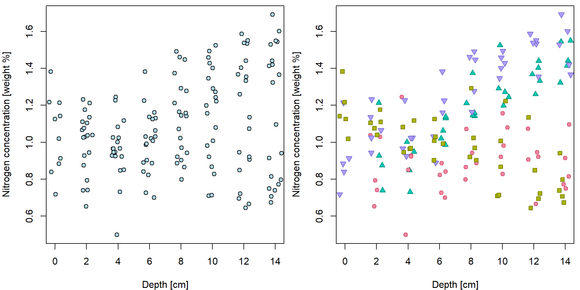 When we do not distinguish groups, we barely see any trend. Fitted line
is only very slowly increasing.
When we do not distinguish groups, we barely see any trend. Fitted line
is only very slowly increasing.
fit1 <- lm(N ~ depth, data = peat)
summary(fit1)
##
## Call:
## lm(formula = N ~ depth, data = peat)
##
## Residuals:
## Min 1Q Median 3Q Max
## -0.52495 -0.17752 -0.00433 0.19054 0.51861
##
## Coefficients:
## Estimate Std. Error t value Pr(>|t|)
## (Intercept) 0.963937 0.040603 23.740 < 2e-16 ***
## depth 0.014969 0.004672 3.204 0.00166 **
## ---
## Signif. codes: 0 '***' 0.001 '**' 0.01 '*' 0.05 '.' 0.1 ' ' 1
##
## Residual standard error: 0.247 on 146 degrees of freedom
## Multiple R-squared: 0.0657, Adjusted R-squared: 0.0593
## F-statistic: 10.27 on 1 and 146 DF, p-value: 0.001663par(mfrow = c(1,1), mar = c(4,4,0.5,0.5))
plot(N ~ jitter(depth), data = peat, pch = 21, bg = "lightblue",
xlab = XLAB, ylab = YLAB, xlim = XLIM, ylim = YLIM)
abline(fit1, col = "darkblue", lwd = 2)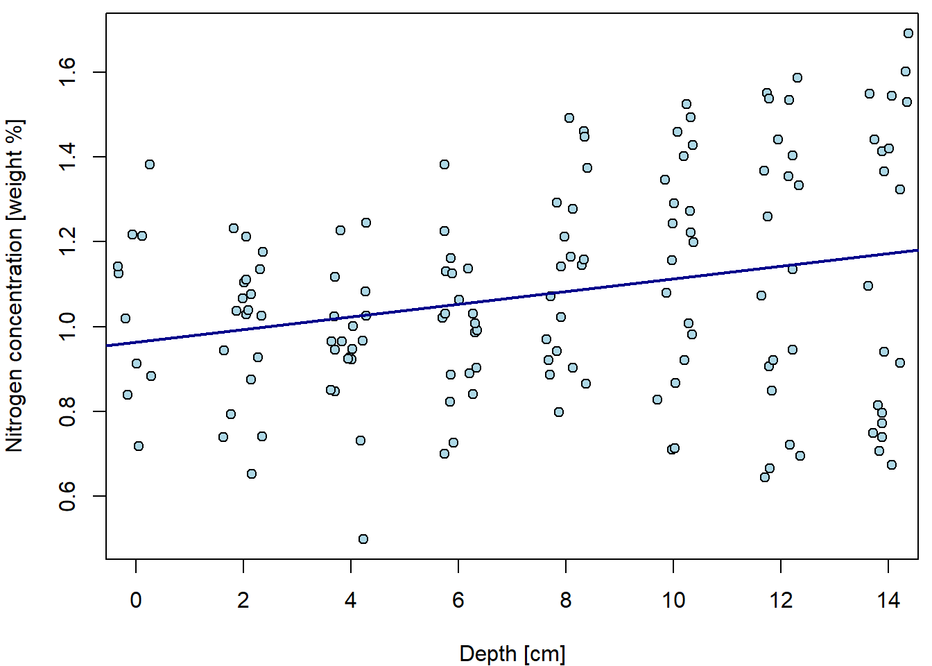
In order to fit line for each group we had to create a subset and estimate line for each subset. We would like to avoid this practice and fit that with one model.
However, additive model is not enough. Remember, additive model leads to parallel lines!
fit2 <- lm(N ~ depth + group, data = peat)
summary(fit2)
##
## Call:
## lm(formula = N ~ depth + group, data = peat)
##
## Residuals:
## Min 1Q Median 3Q Max
## -0.42064 -0.14160 0.01434 0.15407 0.51768
##
## Coefficients:
## Estimate Std. Error t value Pr(>|t|)
## (Intercept) 0.760276 0.044944 16.916 < 2e-16 ***
## depth 0.015883 0.003766 4.218 4.36e-05 ***
## groupCB-VJJ 0.104746 0.045822 2.286 0.0237 *
## groupVJJ 0.297530 0.047888 6.213 5.35e-09 ***
## groupVJJ-CB 0.377879 0.045822 8.247 9.61e-14 ***
## ---
## Signif. codes: 0 '***' 0.001 '**' 0.01 '*' 0.05 '.' 0.1 ' ' 1
##
## Residual standard error: 0.1973 on 143 degrees of freedom
## Multiple R-squared: 0.416, Adjusted R-squared: 0.3996
## F-statistic: 25.46 on 4 and 143 DF, p-value: 6.141e-16par(mfrow = c(1,1), mar = c(4,4,0.5,0.5))
plot(N ~ jitter(depth), data = peat,
pch = PCH[group], col = COL[group], bg = BGC[group],
xlab = XLAB, ylab = YLAB, xlim = XLIM, ylim = YLIM)
intercepts <- coef(fit2)[1] + c(0, coef(fit2)[3:5])
slope <- coef(fit2)[2]
for(g in 1:4){
abline(a = intercepts[g], b = slope, col = DARK[g], lwd = 2)
}
legend("topleft", legend = levels(peat$group), ncol = 2, title = "Group",
col = COL, pch = PCH, pt.bg = BGC, lty = 1, lwd = 2)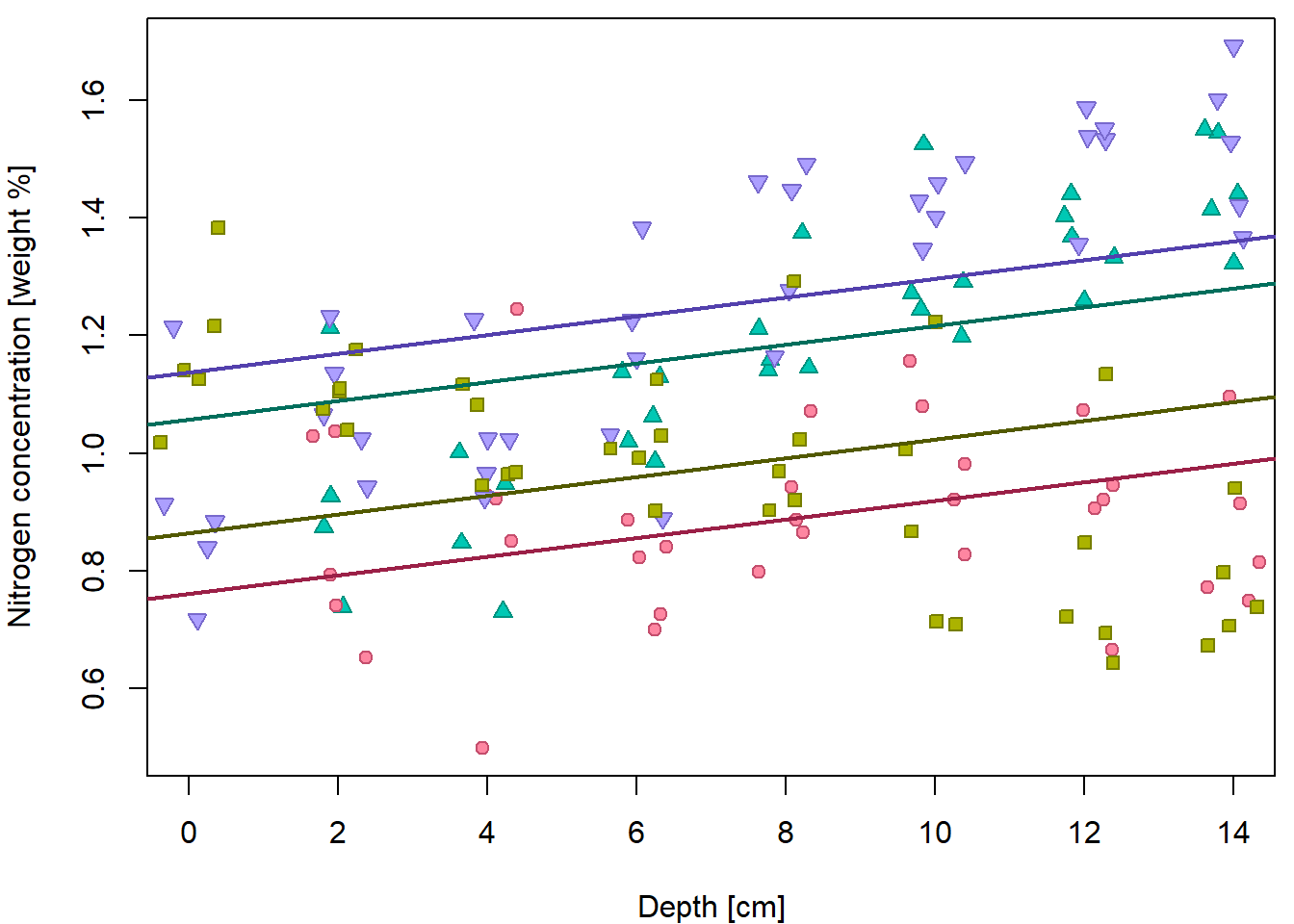 This does not fit the data well. We need specific slopes for each group.
And this is where interactions play the key role.
This does not fit the data well. We need specific slopes for each group.
And this is where interactions play the key role.
An interaction term depth * group in this case leads to
the following model: \[\begin{multline}
\mathsf{E} \left[N | D=d, G=g\right] =
\beta_1
+ \beta_2 d
+ \beta_3 \mathbf{1}(g=\mathtt{CB-VJJ})
+ \beta_4 \mathbf{1}(g=\mathtt{VJJ})
+ \beta_5 \mathbf{1}(g=\mathtt{VJJ-CB})
+ \\
+ \beta_6 d \mathbf{1}(g=\mathtt{CB-VJJ})
+ \beta_7 d \mathbf{1}(g=\mathtt{VJJ})
+ \beta_8 d \mathbf{1}(g=\mathtt{VJJ-CB})
\end{multline}\] Rewriting it for groups separately we have:
\[
\begin{aligned}
\mathsf{E} \left[N | D=d, G=\mathtt{CB}\right]
&= \beta_1 + \beta_2 d
\\
\mathsf{E} \left[N | D=d, G=\mathtt{CB-VJJ}\right]
&= (\beta_1 + \beta_3) + (\beta_2 + \beta_6) d
\\
\mathsf{E} \left[N | D=d, G=\mathtt{VJJ}\right]
&= (\beta_1 + \beta_4) + (\beta_2 + \beta_7) d
\\
\mathsf{E} \left[N | D=d, G=\mathtt{VJJ-CB}\right]
&= (\beta_1 + \beta_5) + (\beta_2 + \beta_8) d
\\
\end{aligned}
\]
fit3 <- lm(N ~ depth * group, data = peat)
summary(fit3)
##
## Call:
## lm(formula = N ~ depth * group, data = peat)
##
## Residuals:
## Min 1Q Median 3Q Max
## -0.36829 -0.08469 -0.00789 0.06112 0.37713
##
## Coefficients:
## Estimate Std. Error t value Pr(>|t|)
## (Intercept) 0.846956 0.051193 16.544 < 2e-16 ***
## depth 0.005048 0.005724 0.882 0.379
## groupCB-VJJ 0.322113 0.064417 5.000 1.68e-06 ***
## groupVJJ -0.064041 0.075374 -0.850 0.397
## groupVJJ-CB 0.075906 0.064417 1.178 0.241
## depth:groupCB-VJJ -0.032600 0.007389 -4.412 2.03e-05 ***
## depth:groupVJJ 0.043942 0.008312 5.287 4.68e-07 ***
## depth:groupVJJ-CB 0.041591 0.007389 5.629 9.56e-08 ***
## ---
## Signif. codes: 0 '***' 0.001 '**' 0.01 '*' 0.05 '.' 0.1 ' ' 1
##
## Residual standard error: 0.1354 on 140 degrees of freedom
## Multiple R-squared: 0.7306, Adjusted R-squared: 0.7171
## F-statistic: 54.23 on 7 and 140 DF, p-value: < 2.2e-16par(mfrow = c(1,1), mar = c(4,4,0.5,0.5))
plot(N ~ jitter(depth), data = peat,
pch = PCH[group], col = COL[group], bg = BGC[group],
xlab = XLAB, ylab = YLAB, xlim = XLIM, ylim = YLIM)
intercepts <- coef(fit3)[1] + c(0, coef(fit3)[3:5])
slopes <- coef(fit3)[2] + c(0, coef(fit3)[6:8])
for(g in 1:4){
abline(a = intercepts[g], b = slopes[g], col = DARK[g], lwd = 2)
}
legend("topleft", legend = levels(peat$group), ncol = 2, title = "Group",
col = COL, pch = PCH, pt.bg = BGC, lty = 1, lwd = 2)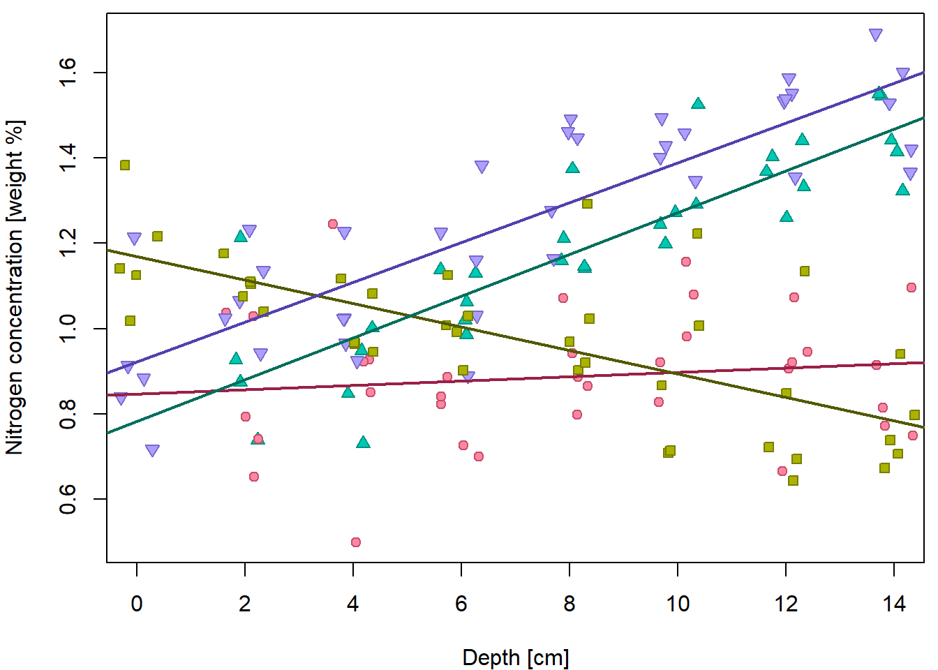
Individual work
- How would you express interaction coefficients in terms of expected values? How would you interpret them?
- What is the difference between the two approaches: a) fit line for each subset of data, b) interaction model in terms of residual variance?
4. Complex model with many regressors and interactions
Now, we will consider another dataset from the mffSM
packages.
Data are provided from the American Association of University Professors
(AAUP) on annual faculty salary survey of American colleges and
universities, 1995.
data(AAUP, package = "mffSM")

dim(AAUP)
## [1] 1161 17head(AAUP)## FICE name state type salary.prof salary.assoc salary.assist salary compens.prof
## 1 1061 Alaska Pacific University AK IIB 454 382 362 382 567
## 2 1063 Univ.Alaska-Fairbanks AK I 686 560 432 508 914
## 3 1065 Univ.Alaska-Southeast AK IIA 533 494 329 415 716
## 4 11462 Univ.Alaska-Anchorage AK IIA 612 507 414 498 825
## 5 1002 Alabama Agri.&Mech. Univ. AL IIA 442 369 310 350 530
## 6 1004 University of Montevallo AL IIA 441 385 310 388 542
## compens.assoc compens.assist compens n.prof n.assoc n.assist n.instruct n.faculty
## 1 485 471 487 6 11 9 4 32
## 2 753 572 677 74 125 118 40 404
## 3 663 442 559 9 26 20 9 70
## 4 681 557 670 115 124 101 21 392
## 5 444 376 423 59 77 102 24 262
## 6 473 383 477 57 33 35 2 127summary(AAUP)## FICE name state type salary.prof salary.assoc salary.assist
## Min. : 1002 Length:1161 PA : 85 I :180 Min. : 270.0 Min. :234.0 Min. :199.0
## 1st Qu.: 1903 Class :character NY : 81 IIA:363 1st Qu.: 440.0 1st Qu.:367.0 1st Qu.:313.0
## Median : 2668 Mode :character CA : 54 IIB:618 Median : 506.0 Median :413.0 Median :349.0
## Mean : 3052 TX : 54 Mean : 524.1 Mean :416.4 Mean :351.9
## 3rd Qu.: 3420 OH : 53 3rd Qu.: 600.0 3rd Qu.:461.0 3rd Qu.:388.0
## Max. :29269 IL : 50 Max. :1009.0 Max. :733.0 Max. :576.0
## (Other):784 NA's :68 NA's :36 NA's :24
## salary compens.prof compens.assoc compens.assist compens n.prof
## Min. :232.0 Min. : 319.0 Min. :292.0 Min. :246.0 Min. : 265.0 Min. : 0.0
## 1st Qu.:352.0 1st Qu.: 547.0 1st Qu.:456.0 1st Qu.:389.0 1st Qu.: 436.0 1st Qu.: 18.0
## Median :407.0 Median : 635.0 Median :519.0 Median :437.0 Median : 510.0 Median : 40.0
## Mean :420.4 Mean : 653.5 Mean :523.8 Mean :442.1 Mean : 526.7 Mean : 95.1
## 3rd Qu.:475.0 3rd Qu.: 753.0 3rd Qu.:583.0 3rd Qu.:493.0 3rd Qu.: 600.0 3rd Qu.:105.0
## Max. :866.0 Max. :1236.0 Max. :909.0 Max. :717.0 Max. :1075.0 Max. :997.0
## NA's :68 NA's :36 NA's :24
## n.assoc n.assist n.instruct n.faculty
## Min. : 0.00 Min. : 0.00 Min. : 0.00 Min. : 7.0
## 1st Qu.: 19.00 1st Qu.: 21.00 1st Qu.: 2.00 1st Qu.: 68.0
## Median : 38.00 Median : 40.00 Median : 6.00 Median : 132.0
## Mean : 72.39 Mean : 68.63 Mean : 12.74 Mean : 257.4
## 3rd Qu.: 89.00 3rd Qu.: 92.00 3rd Qu.: 14.00 3rd Qu.: 323.0
## Max. :721.00 Max. :510.00 Max. :178.00 Max. :2261.0
## ### A data subset containing only relevant variables
aaup <- subset(AAUP, select = c("FICE", "name", "state", "type", "n.prof",
"n.assoc", "n.assist", "salary.assoc"))
dim(aaup)## [1] 1161 8head(aaup)## FICE name state type n.prof n.assoc n.assist salary.assoc
## 1 1061 Alaska Pacific University AK IIB 6 11 9 382
## 2 1063 Univ.Alaska-Fairbanks AK I 74 125 118 560
## 3 1065 Univ.Alaska-Southeast AK IIA 9 26 20 494
## 4 11462 Univ.Alaska-Anchorage AK IIA 115 124 101 507
## 5 1002 Alabama Agri.&Mech. Univ. AL IIA 59 77 102 369
## 6 1004 University of Montevallo AL IIA 57 33 35 385summary(aaup)## FICE name state type n.prof n.assoc n.assist
## Min. : 1002 Length:1161 PA : 85 I :180 Min. : 0.0 Min. : 0.00 Min. : 0.00
## 1st Qu.: 1903 Class :character NY : 81 IIA:363 1st Qu.: 18.0 1st Qu.: 19.00 1st Qu.: 21.00
## Median : 2668 Mode :character CA : 54 IIB:618 Median : 40.0 Median : 38.00 Median : 40.00
## Mean : 3052 TX : 54 Mean : 95.1 Mean : 72.39 Mean : 68.63
## 3rd Qu.: 3420 OH : 53 3rd Qu.:105.0 3rd Qu.: 89.00 3rd Qu.: 92.00
## Max. :29269 IL : 50 Max. :997.0 Max. :721.00 Max. :510.00
## (Other):784
## salary.assoc
## Min. :234.0
## 1st Qu.:367.0
## Median :413.0
## Mean :416.4
## 3rd Qu.:461.0
## Max. :733.0
## NA's :36### considering only a subset of covariates
Data <- subset(aaup,
complete.cases(aaup[, c("salary.assoc", "n.prof", "n.assoc", "n.assist", "type")]))Individual work
- Consider the dataset on annual income of university professors in USA and perform simple exploratory analysis.
- Focus on average yearly salaries for different types of the universities.
- In our exploratory analysis try to take into account also an information about different numbers of university professors (of different ranks) at the given university.
COL3 <- rainbow_hcl(3)
plot(salary.assoc ~ type, data = aaup,
     xlab = "Type of institution",  ylab = "Salary associate professor [USD 100]",
     col = COL3)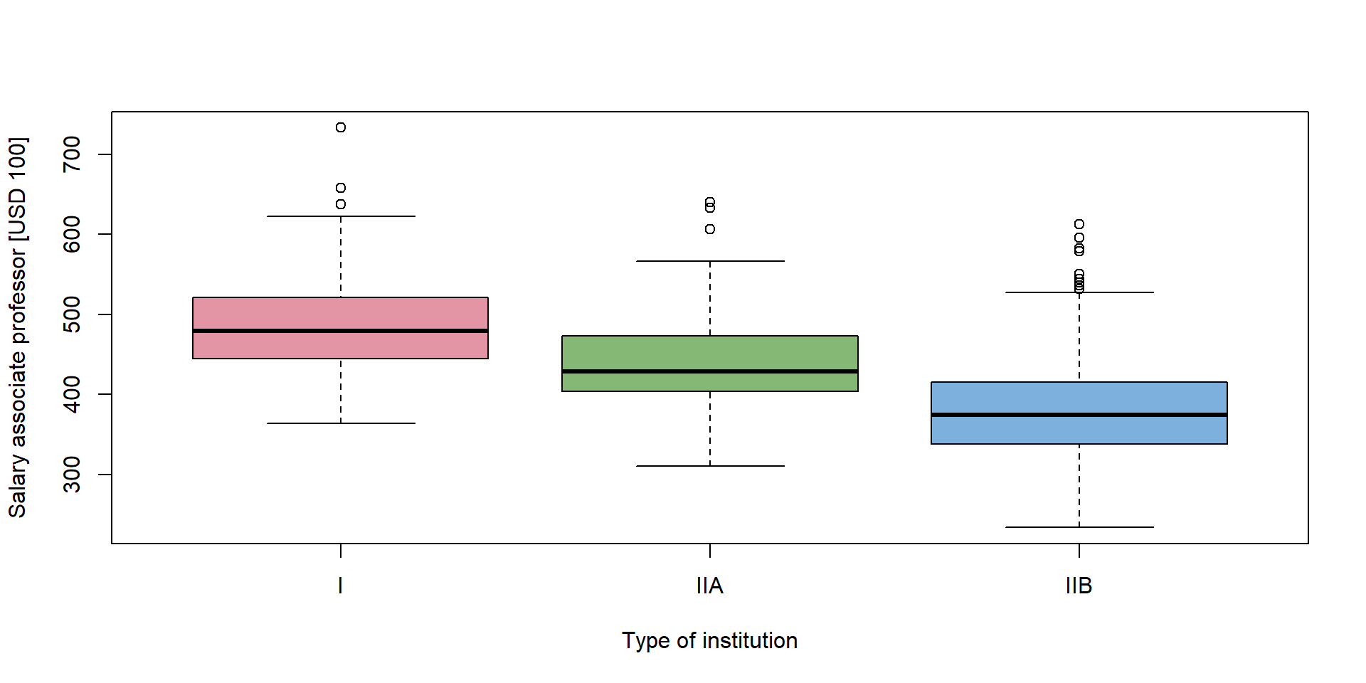
We will fit a few different models that we will compare later. Firstly, a simple additive model:
summary(m1orig <- lm(salary.assoc ~ type + n.prof + n.assoc + n.assist, data = Data))##
## Call:
## lm(formula = salary.assoc ~ type + n.prof + n.assoc + n.assist,
## data = Data)
##
## Residuals:
## Min 1Q Median 3Q Max
## -144.657 -39.679 -6.887 33.560 266.641
##
## Coefficients:
## Estimate Std. Error t value Pr(>|t|)
## (Intercept) 448.49675 8.61850 52.039 < 2e-16 ***
## typeIIA -19.45462 7.18979 -2.706 0.00692 **
## typeIIB -70.56945 8.20735 -8.598 < 2e-16 ***
## n.prof 0.10370 0.02760 3.758 0.00018 ***
## n.assoc 0.07075 0.05883 1.203 0.22940
## n.assist -0.06609 0.06445 -1.025 0.30538
## ---
## Signif. codes: 0 '***' 0.001 '**' 0.01 '*' 0.05 '.' 0.1 ' ' 1
##
## Residual standard error: 58.21 on 1119 degrees of freedom
## Multiple R-squared: 0.3408, Adjusted R-squared: 0.3379
## F-statistic: 115.7 on 5 and 1119 DF, p-value: < 2.2e-16Interpret the estimated parameters in the model and compare it with the interpretation of the estimated parameters in the following model:
Data <- transform(Data, n.prof40 = n.prof - 40,
                  n.assoc40 = n.assoc - 40,
                  n.assist40 = n.assist - 40)
summary(m1 <- lm(salary.assoc ~ type + n.prof40 + n.assoc40 + n.assist40, data = Data))
##
## Call:
## lm(formula = salary.assoc ~ type + n.prof40 + n.assoc40 + n.assist40,
## data = Data)
##
## Residuals:
## Min 1Q Median 3Q Max
## -144.657 -39.679 -6.887 33.560 266.641
##
## Coefficients:
## Estimate Std. Error t value Pr(>|t|)
## (Intercept) 452.83099 7.50270 60.356 < 2e-16 ***
## typeIIA -19.45462 7.18979 -2.706 0.00692 **
## typeIIB -70.56945 8.20735 -8.598 < 2e-16 ***
## n.prof40 0.10370 0.02760 3.758 0.00018 ***
## n.assoc40 0.07075 0.05883 1.203 0.22940
## n.assist40 -0.06609 0.06445 -1.025 0.30538
## ---
## Signif. codes: 0 '***' 0.001 '**' 0.01 '*' 0.05 '.' 0.1 ' ' 1
##
## Residual standard error: 58.21 on 1119 degrees of freedom
## Multiple R-squared: 0.3408, Adjusted R-squared: 0.3379
## F-statistic: 115.7 on 5 and 1119 DF, p-value: < 2.2e-16And, once more the same model, however, with a different
parametrization (contr.sum) used for the categorical
covariate of the university type:
m1B <- lm(salary.assoc ~ type + n.prof40 + n.assoc40 + n.assist40, data = Data,
          contrasts = list(type = "contr.sum"))
Finally, one more complicated model with interactions (in two different parametrization of the continuous covariates):
summary(m2orig <- lm(salary.assoc ~ type + n.prof*n.assoc + n.assist, data = Data)) ##
## Call:
## lm(formula = salary.assoc ~ type + n.prof * n.assoc + n.assist,
## data = Data)
##
## Residuals:
## Min 1Q Median 3Q Max
## -137.779 -39.956 -6.683 33.105 280.196
##
## Coefficients:
## Estimate Std. Error t value Pr(>|t|)
## (Intercept) 3.946e+02 9.949e+00 39.662 < 2e-16 ***
## typeIIA 1.697e+00 7.237e+00 0.235 0.81461
## typeIIB -2.828e+01 8.994e+00 -3.144 0.00171 **
## n.prof 3.079e-01 3.376e-02 9.119 < 2e-16 ***
## n.assoc 4.171e-01 6.671e-02 6.252 5.76e-10 ***
## n.assist -1.339e-01 6.229e-02 -2.150 0.03175 *
## n.prof:n.assoc -8.444e-04 8.649e-05 -9.763 < 2e-16 ***
## ---
## Signif. codes: 0 '***' 0.001 '**' 0.01 '*' 0.05 '.' 0.1 ' ' 1
##
## Residual standard error: 55.91 on 1118 degrees of freedom
## Multiple R-squared: 0.3926, Adjusted R-squared: 0.3894
## F-statistic: 120.5 on 6 and 1118 DF, p-value: < 2.2e-16summary(m2 <- lm(salary.assoc ~ type + n.prof40*n.assoc40 + n.assist40, data = Data)) ##
## Call:
## lm(formula = salary.assoc ~ type + n.prof40 * n.assoc40 + n.assist40,
## data = Data)
##
## Residuals:
## Min 1Q Median 3Q Max
## -137.779 -39.956 -6.683 33.105 280.196
##
## Coefficients:
## Estimate Std. Error t value Pr(>|t|)
## (Intercept) 4.169e+02 8.091e+00 51.522 < 2e-16 ***
## typeIIA 1.697e+00 7.237e+00 0.235 0.81461
## typeIIB -2.828e+01 8.994e+00 -3.144 0.00171 **
## n.prof40 2.741e-01 3.173e-02 8.637 < 2e-16 ***
## n.assoc40 3.833e-01 6.494e-02 5.903 4.74e-09 ***
## n.assist40 -1.339e-01 6.229e-02 -2.150 0.03175 *
## n.prof40:n.assoc40 -8.444e-04 8.649e-05 -9.763 < 2e-16 ***
## ---
## Signif. codes: 0 '***' 0.001 '**' 0.01 '*' 0.05 '.' 0.1 ' ' 1
##
## Residual standard error: 55.91 on 1118 degrees of freedom
## Multiple R-squared: 0.3926, Adjusted R-squared: 0.3894
## F-statistic: 120.5 on 6 and 1118 DF, p-value: < 2.2e-16Individual work
- Compare both models and interpret the estimated parameters.
- Focus on the estimated salaries for different types of university while controlling for specific amounts of the academic personel at the given university.
5. Hierarchical structure of the model
Finally, we will briefly compare a hierarchically well formulated model and a model that is non-hierarchical, Above, we already considered the model for the expected anual salary of the university professors in the USA and the proportion of the professors, associate professors and assistant professors were lowered by 40 (in order to ensure a better interpretation of the intercept parameter and better interpretation of the interaction terms).
Consider firstly a hierarchically well formulated model with and without the corresponding linear transformation of the number of professors.
summary(m3orig <- lm(salary.assoc ~ type + n.assoc * n.prof, data = Data)) ##
## Call:
## lm(formula = salary.assoc ~ type + n.assoc * n.prof, data = Data)
##
## Residuals:
## Min 1Q Median 3Q Max
## -137.782 -40.497 -6.265 33.621 283.148
##
## Coefficients:
## Estimate Std. Error t value Pr(>|t|)
## (Intercept) 3.918e+02 9.883e+00 39.651 < 2e-16 ***
## typeIIA 1.750e+00 7.248e+00 0.241 0.80924
## typeIIB -2.684e+01 8.983e+00 -2.988 0.00287 **
## n.assoc 3.340e-01 5.447e-02 6.132 1.2e-09 ***
## n.prof 2.910e-01 3.289e-02 8.848 < 2e-16 ***
## n.assoc:n.prof -8.236e-04 8.609e-05 -9.568 < 2e-16 ***
## ---
## Signif. codes: 0 '***' 0.001 '**' 0.01 '*' 0.05 '.' 0.1 ' ' 1
##
## Residual standard error: 56 on 1119 degrees of freedom
## Multiple R-squared: 0.3901, Adjusted R-squared: 0.3874
## F-statistic: 143.2 on 5 and 1119 DF, p-value: < 2.2e-16summary(m3 <- lm(salary.assoc ~ type + n.assoc40 * n.prof40, data = Data)) ##
## Call:
## lm(formula = salary.assoc ~ type + n.assoc40 * n.prof40, data = Data)
##
## Residuals:
## Min 1Q Median 3Q Max
## -137.782 -40.497 -6.265 33.621 283.148
##
## Coefficients:
## Estimate Std. Error t value Pr(>|t|)
## (Intercept) 4.155e+02 8.080e+00 51.428 < 2e-16 ***
## typeIIA 1.750e+00 7.248e+00 0.241 0.80924
## typeIIB -2.684e+01 8.983e+00 -2.988 0.00287 **
## n.assoc40 3.010e-01 5.256e-02 5.728 1.31e-08 ***
## n.prof40 2.581e-01 3.090e-02 8.353 < 2e-16 ***
## n.assoc40:n.prof40 -8.236e-04 8.609e-05 -9.568 < 2e-16 ***
## ---
## Signif. codes: 0 '***' 0.001 '**' 0.01 '*' 0.05 '.' 0.1 ' ' 1
##
## Residual standard error: 56 on 1119 degrees of freedom
## Multiple R-squared: 0.3901, Adjusted R-squared: 0.3874
## F-statistic: 143.2 on 5 and 1119 DF, p-value: < 2.2e-16Individual work
Both models above a hierarchically well formulated models.
- Compare the estimated parameters and try to reconstruct the parameter estimates from one model using the estimates from the second model.
- Compare summary statistics for both models (i.e., degrees of freedom, residual sum of squares, \(F\)-statistic, etc. )
Now, we will fit two very similar models but both will be non-hierarchical. Compare both models and try to understand the effect of the transformation used.
summary(m3orig <- lm(salary.assoc ~ - 1 + type + n.assoc * n.prof - n.prof, data = Data)) ##
## Call:
## lm(formula = salary.assoc ~ -1 + type + n.assoc * n.prof - n.prof,
## data = Data)
##
## Residuals:
## Min 1Q Median 3Q Max
## -141.166 -40.814 -7.942 33.808 288.497
##
## Coefficients:
## Estimate Std. Error t value Pr(>|t|)
## typeI 4.312e+02 9.122e+00 47.272 < 2e-16 ***
## typeIIA 4.120e+02 4.869e+00 84.621 < 2e-16 ***
## typeIIB 3.709e+02 2.763e+00 134.221 < 2e-16 ***
## n.assoc 3.933e-01 5.589e-02 7.037 3.41e-12 ***
## n.assoc:n.prof -3.559e-04 7.025e-05 -5.067 4.73e-07 ***
## ---
## Signif. codes: 0 '***' 0.001 '**' 0.01 '*' 0.05 '.' 0.1 ' ' 1
##
## Residual standard error: 57.9 on 1120 degrees of freedom
## Multiple R-squared: 0.9813, Adjusted R-squared: 0.9812
## F-statistic: 1.176e+04 on 5 and 1120 DF, p-value: < 2.2e-16summary(m3 <- lm(salary.assoc ~ - 1 + type + n.assoc40 * n.prof40 - n.prof40, data = Data)) ##
## Call:
## lm(formula = salary.assoc ~ -1 + type + n.assoc40 * n.prof40 -
## n.prof40, data = Data)
##
## Residuals:
## Min 1Q Median 3Q Max
## -140.522 -40.753 -7.787 34.716 289.971
##
## Coefficients:
## Estimate Std. Error t value Pr(>|t|)
## typeI 4.430e+02 7.602e+00 58.280 < 2e-16 ***
## typeIIA 4.258e+02 3.496e+00 121.800 < 2e-16 ***
## typeIIB 3.866e+02 2.512e+00 153.892 < 2e-16 ***
## n.assoc40 4.055e-01 5.259e-02 7.710 2.77e-14 ***
## n.assoc40:n.prof40 -4.337e-04 7.452e-05 -5.821 7.65e-09 ***
## ---
## Signif. codes: 0 '***' 0.001 '**' 0.01 '*' 0.05 '.' 0.1 ' ' 1
##
## Residual standard error: 57.69 on 1120 degrees of freedom
## Multiple R-squared: 0.9814, Adjusted R-squared: 0.9814
## F-statistic: 1.184e+04 on 5 and 1120 DF, p-value: < 2.2e-166. Finding suitable hierarchically well-formulated model
We will apply stepwise backward selection process and start with model containing all interactions of second order
summary(mfull <- lm(salary.assoc ~ (type + n.prof40 + n.assoc40 + n.assist40)^2, data = Data)) ##
## Call:
## lm(formula = salary.assoc ~ (type + n.prof40 + n.assoc40 + n.assist40)^2,
## data = Data)
##
## Residuals:
## Min 1Q Median 3Q Max
## -187.745 -35.767 -4.398 29.689 212.118
##
## Coefficients:
## Estimate Std. Error t value Pr(>|t|)
## (Intercept) 4.722e+02 1.190e+01 39.674 < 2e-16 ***
## typeIIA -4.442e+01 1.225e+01 -3.625 0.000302 ***
## typeIIB -6.568e+01 1.230e+01 -5.340 1.12e-07 ***
## n.prof40 4.086e-01 7.086e-02 5.767 1.05e-08 ***
## n.assoc40 1.299e-01 1.296e-01 1.002 0.316368
## n.assist40 -7.585e-01 1.673e-01 -4.534 6.42e-06 ***
## typeIIA:n.prof40 -2.825e-01 6.967e-02 -4.054 5.38e-05 ***
## typeIIB:n.prof40 3.599e-01 1.518e-01 2.371 0.017895 *
## typeIIA:n.assoc40 4.866e-01 1.583e-01 3.073 0.002168 **
## typeIIB:n.assoc40 7.603e-01 2.428e-01 3.131 0.001785 **
## typeIIA:n.assist40 2.597e-01 1.680e-01 1.545 0.122542
## typeIIB:n.assist40 1.050e+00 2.346e-01 4.473 8.50e-06 ***
## n.prof40:n.assoc40 -1.246e-03 2.863e-04 -4.352 1.47e-05 ***
## n.prof40:n.assist40 2.462e-04 3.229e-04 0.763 0.445830
## n.assoc40:n.assist40 1.649e-03 5.306e-04 3.108 0.001931 **
## ---
## Signif. codes: 0 '***' 0.001 '**' 0.01 '*' 0.05 '.' 0.1 ' ' 1
##
## Residual standard error: 51.67 on 1110 degrees of freedom
## Multiple R-squared: 0.485, Adjusted R-squared: 0.4785
## F-statistic: 74.66 on 14 and 1110 DF, p-value: < 2.2e-16You can check which covariates to drop with:
drop1(mfull, test = "F")## Single term deletions
##
## Model:
## salary.assoc ~ (type + n.prof40 + n.assoc40 + n.assist40)^2
## Df Sum of Sq RSS AIC F value Pr(>F)
## <none> 2963012 8890.7
## type:n.prof40 2 86497 3049509 8919.1 16.2017 1.160e-07 ***
## type:n.assoc40 2 37467 3000479 8900.8 7.0179 0.000936 ***
## type:n.assist40 2 57827 3020839 8908.4 10.8316 2.194e-05 ***
## n.prof40:n.assoc40 1 50555 3013567 8907.7 18.9387 1.474e-05 ***
## n.prof40:n.assist40 1 1553 2964565 8889.3 0.5816 0.445830
## n.assoc40:n.assist40 1 25785 2988798 8898.4 9.6597 0.001931 **
## ---
## Signif. codes: 0 '***' 0.001 '**' 0.01 '*' 0.05 '.' 0.1 ' ' 1We can update the model by eliminating insignificant terms:
m4 <- update(mfull, .~.-n.prof40:n.assist40)
drop1(m4, test = "F")
## Single term deletions
##
## Model:
## salary.assoc ~ type + n.prof40 + n.assoc40 + n.assist40 + type:n.prof40 +
## type:n.assoc40 + type:n.assist40 + n.prof40:n.assoc40 + n.assoc40:n.assist40
## Df Sum of Sq RSS AIC F value Pr(>F)
## <none> 2964565 8889.3
## type:n.prof40 2 98228 3062793 8922.0 18.406 1.368e-08 ***
## type:n.assoc40 2 67205 3031770 8910.5 12.593 3.909e-06 ***
## type:n.assist40 2 57329 3021894 8906.8 10.742 2.394e-05 ***
## n.prof40:n.assoc40 1 55991 3020556 8908.3 20.983 5.157e-06 ***
## n.assoc40:n.assist40 1 34025 2998589 8900.1 12.751 0.000371 ***
## ---
## Signif. codes: 0 '***' 0.001 '**' 0.01 '*' 0.05 '.' 0.1 ' ' 1Compare different models and submodels
anova(m1, m4, test = "F") # improvement## Analysis of Variance Table
##
## Model 1: salary.assoc ~ type + n.prof40 + n.assoc40 + n.assist40
## Model 2: salary.assoc ~ type + n.prof40 + n.assoc40 + n.assist40 + type:n.prof40 +
## type:n.assoc40 + type:n.assist40 + n.prof40:n.assoc40 + n.assoc40:n.assist40
## Res.Df RSS Df Sum of Sq F Pr(>F)
## 1 1119 3792157
## 2 1111 2964565 8 827592 38.769 < 2.2e-16 ***
## ---
## Signif. codes: 0 '***' 0.001 '**' 0.01 '*' 0.05 '.' 0.1 ' ' 1anova(m4, mfull, test = "F") # comparable## Analysis of Variance Table
##
## Model 1: salary.assoc ~ type + n.prof40 + n.assoc40 + n.assist40 + type:n.prof40 +
## type:n.assoc40 + type:n.assist40 + n.prof40:n.assoc40 + n.assoc40:n.assist40
## Model 2: salary.assoc ~ (type + n.prof40 + n.assoc40 + n.assist40)^2
## Res.Df RSS Df Sum of Sq F Pr(>F)
## 1 1111 2964565
## 2 1110 2963012 1 1552.6 0.5816 0.4458add1(m4, scope = "n.prof40:n.assist40", test = "F") # the same - for forward selection## Single term additions
##
## Model:
## salary.assoc ~ type + n.prof40 + n.assoc40 + n.assist40 + type:n.prof40 +
## type:n.assoc40 + type:n.assist40 + n.prof40:n.assoc40 + n.assoc40:n.assist40
## Df Sum of Sq RSS AIC F value Pr(>F)
## <none> 2964565 8889.3
## n.prof40:n.assist40 1 1552.6 2963012 8890.7 0.5816 0.4458