Introduction to fitting linear models
Jan Vávra
Exercise 2
Download this R markdown as: R, Rmd.
Loading the data and libraries
library("mffSM")
library("colorspace")
We want to examine a nitrogen concentration measured at various
depths of the peat. Load the data peat below and try to
understand the design of the underlying experiment. Focus on various
depths in particular.
peat <- read.csv("http://www.karlin.mff.cuni.cz/~vavraj/nmfm334/data/peat.csv",
header = TRUE, stringsAsFactors = TRUE)dim(peat)## [1] 148 3str(peat)## 'data.frame': 148 obs. of 3 variables:
## $ group: Factor w/ 4 levels "CB","CB-VJJ",..: 3 3 3 3 3 3 3 3 3 3 ...
## $ N : num 0.738 0.847 1.063 1.142 1.272 ...
## $ depth: int 2 4 6 8 10 12 14 2 4 6 ...head(peat)## group N depth
## 1 VJJ 0.7383710 2
## 2 VJJ 0.8473675 4
## 3 VJJ 1.0629922 6
## 4 VJJ 1.1419428 8
## 5 VJJ 1.2721831 10
## 6 VJJ 1.4032890 12summary(peat)## group N depth
## CB :35 Min. :0.4989 Min. : 0.000
## CB-VJJ:40 1st Qu.:0.8992 1st Qu.: 4.000
## VJJ :33 Median :1.0343 Median : 8.000
## VJJ-CB:40 Mean :1.0766 Mean : 7.527
## 3rd Qu.:1.2440 3rd Qu.:12.000
## Max. :1.6921 Max. :14.000Visual exploration
Basic scatterplot for Nitrogen concentration given depth:
XLAB <- "Depth [cm]"
YLAB <- "Nitrogen concentration [weight %]"

XLIM <- range(peat[, "depth"])
YLIM <- range(peat[, "N"])

par(mfrow = c(1,1), mar = c(4,4,0.5,0.5))
plot(N ~ depth, data = peat, pch = 21, bg = "lightblue",
     xlab = XLAB, ylab = YLAB, xlim = XLIM, ylim = YLIM)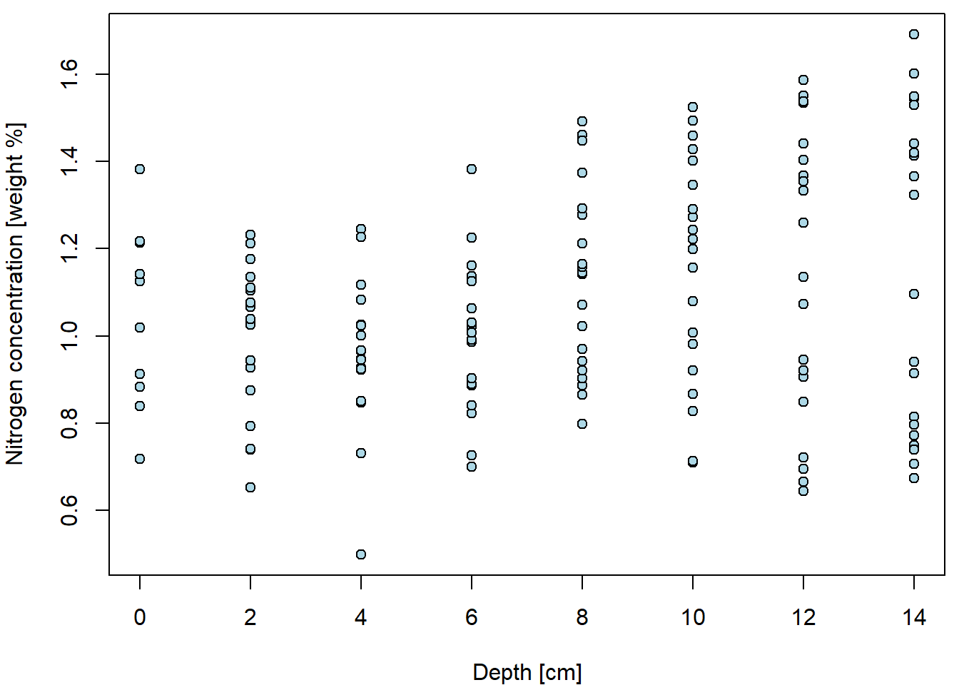
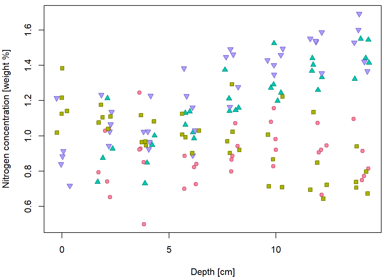
But it can be done better… by distinguishing for different peat types
(variable group).
Groups <- levels(peat[, "group"])
print(Groups)
## [1] "CB" "CB-VJJ" "VJJ" "VJJ-CB"PCH <- c(21, 22, 24, 25)
DARK <- rainbow_hcl(4, c = 80, l = 35)
COL <- rainbow_hcl(4, c = 80, l = 50)
BGC <- rainbow_hcl(4, c = 80, l = 70)
names(PCH) <- names(DARK) <- names(COL) <- names(BGC) <- Groups
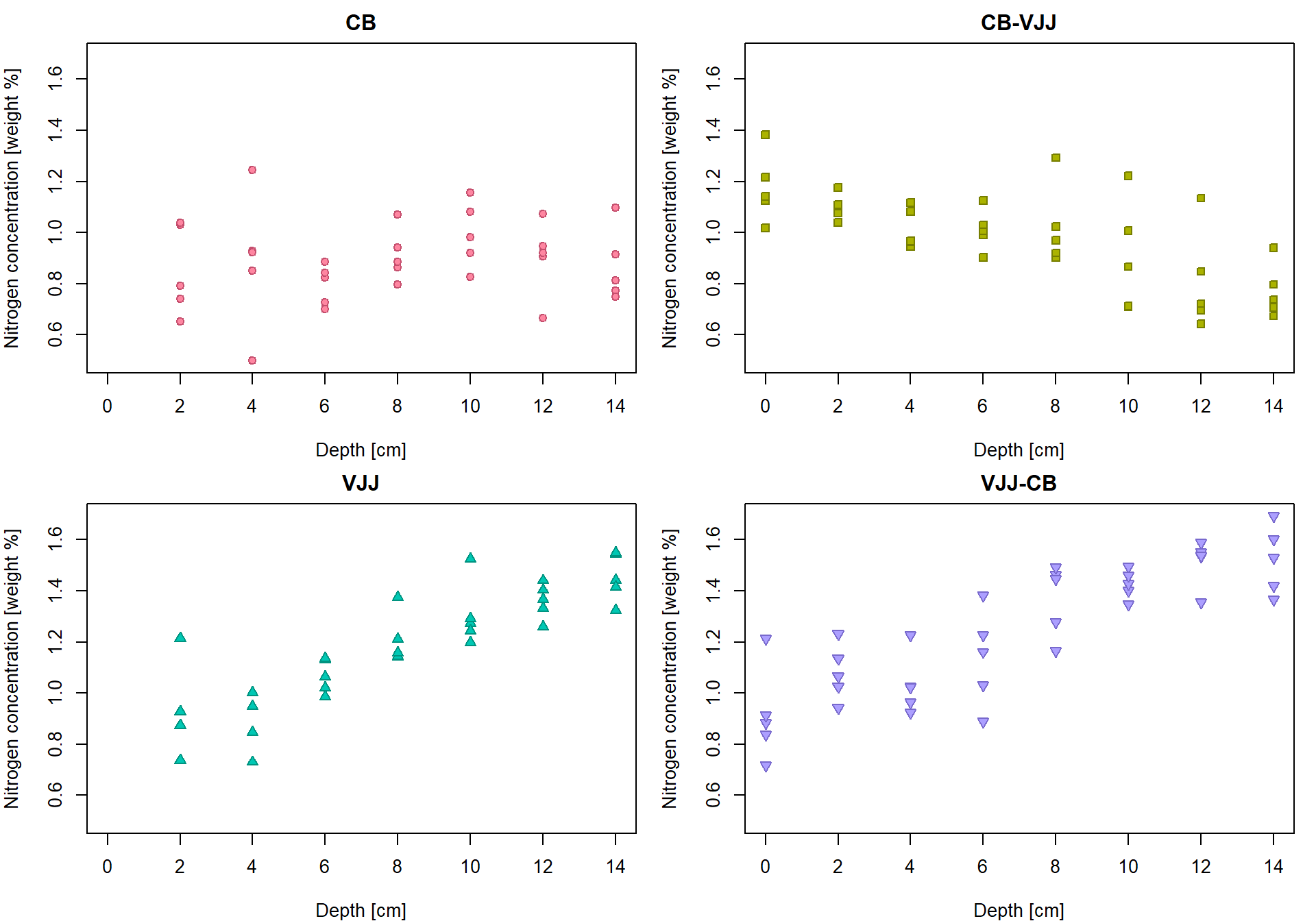
par(mfrow = c(2,2), mar = c(4,4,2,1))
for(g in Groups){
plot(N ~ depth, data = subset(peat, group == g),
pch = PCH[g], col = COL[g], bg = BGC[g],
xlab = XLAB, ylab = YLAB, main = g, xlim = XLIM, ylim = YLIM)
} 
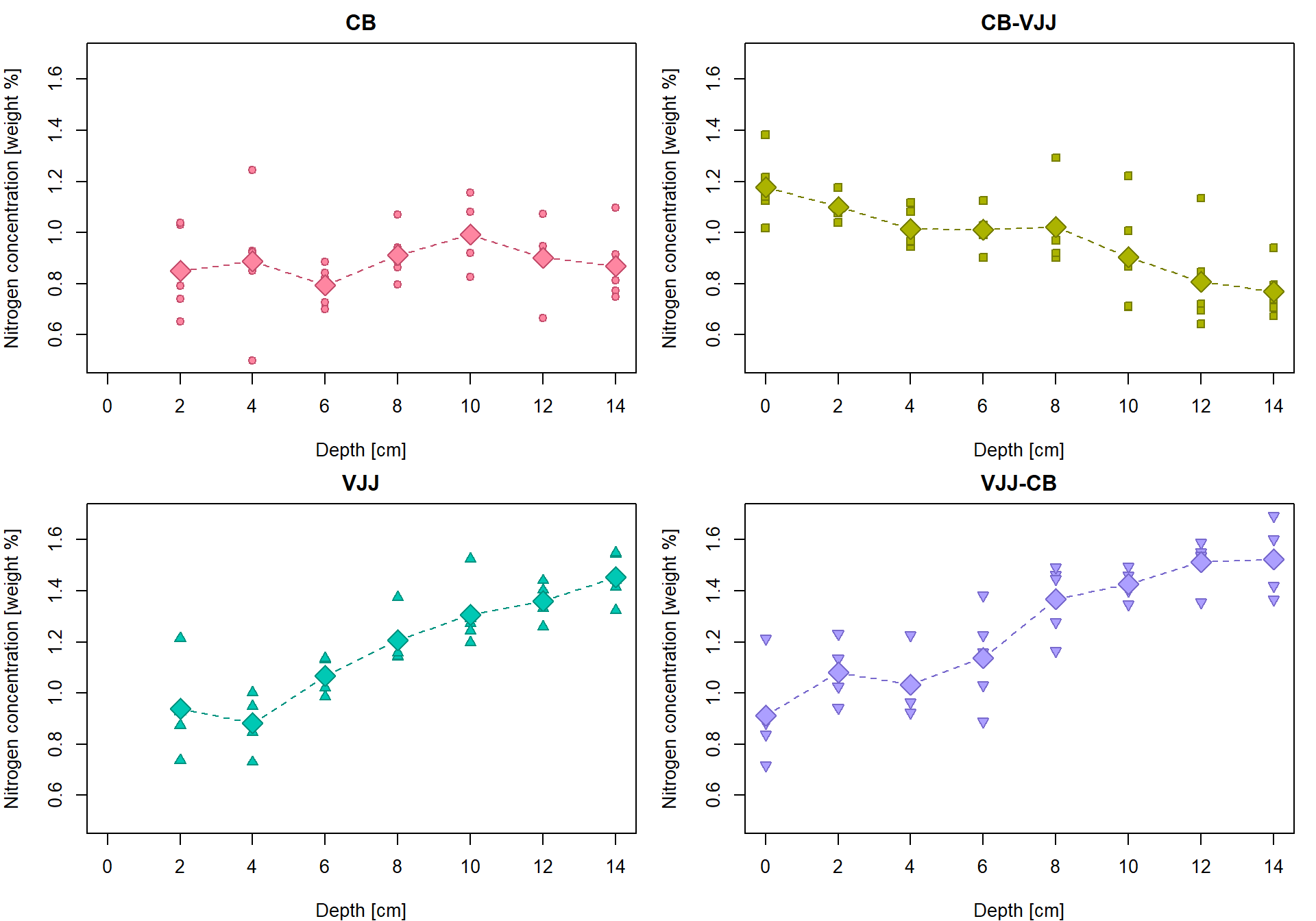
Conditional empirical characteristics by groups
tabs <- list()
# g <- 1 # run for one g
for(g in 1:length(Groups)){
  # data subset containing only the g-th group
  subdata <- subset(peat, group == Groups[g])
  # averages for particular depths
  Mean    <- with(subdata, tapply(N, depth, mean))
  # standard deviations for particular depths
  StdDev  <- with(subdata, tapply(N, depth, sd))
  # numbers of observations for particular depths
  ns      <- with(subdata, tapply(N, depth, length))

  # cat("\n",Groups[g],"\n")
  # print(Mean)
  # print(StdDev)
  # print(ns)

  tabs[[g]] <- data.frame(Depth = as.numeric(names(Mean)),
                          Mean = Mean,
                          Std.Dev = StdDev,
                          n = ns)
  rownames(tabs[[g]]) <- 1:nrow(tabs[[g]])
}
names(tabs) <- Groups
print(tabs)
## $CB
## Depth Mean Std.Dev n
## 1 2 0.8504320 0.17437100 5
## 2 4 0.8885866 0.26575319 5
## 3 6 0.7951133 0.07905635 5
## 4 8 0.9122869 0.10257331 5
## 5 10 0.9930867 0.12950782 5
## 6 12 0.9024869 0.14771465 5
## 7 14 0.8694117 0.14202920 5
##
## $`CB-VJJ`
## Depth Mean Std.Dev n
## 1 0 1.1769177 0.13512002 5
## 2 2 1.1011507 0.05042430 5
## 3 4 1.0153398 0.07849447 5
## 4 6 1.0113715 0.08000427 5
## 5 8 1.0215852 0.15842290 5
## 6 10 0.9036023 0.21677703 5
## 7 12 0.8086419 0.19742942 5
## 8 14 0.7710349 0.10510728 5
##
## $VJJ
## Depth Mean Std.Dev n
## 1 2 0.9381259 0.19972666 4
## 2 4 0.8817402 0.11941469 4
## 3 6 1.0673126 0.06671083 5
## 4 8 1.2065316 0.09810094 5
## 5 10 1.3061741 0.12734137 5
## 6 12 1.3610624 0.06927207 5
## 7 14 1.4549562 0.09526403 5
##
## $`VJJ-CB`
## Depth Mean Std.Dev n
## 1 0 0.9132266 0.18371658 5
## 2 2 1.0804183 0.10997845 5
## 3 4 1.0331289 0.11638281 5
## 4 6 1.1380384 0.18806905 5
## 5 8 1.3685547 0.14144116 5
## 6 10 1.4260073 0.05603573 5
## 7 12 1.5131996 0.09093290 5
## 8 14 1.5221417 0.13197782 5Insert the group averages into the original plot
par(mfrow = c(2,2), mar = c(4,4,2,1))
for (g in Groups){
  plot(N ~ depth, data = subset(peat, group == g),
       pch = PCH[g], col = COL[g], bg = BGC[g],
       xlab = XLAB, ylab = YLAB, main = g, xlim = XLIM, ylim = YLIM)
  lines(tabs[[g]][, "Depth"], tabs[[g]][, "Mean"], type = "b",
        pch = 23, lty = 2, cex = 2, col = COL[g], bg = BGC[g])
} 
Linear regression line for the group “CB-VJJ”
g <- "CB-VJJ"
n <- sum(peat$group == g)
We will assume a linear relationship between depth and Nitrogen
concentration for each group separately. First, we focus on
group CB-VJJ. Let \(Y_i\) be the
Nitrogen concentration measured in depth \(X_i\), where \(i\) is the index of the observation.
Then,
\[ Y_i = a + b X_i + \varepsilon_i \qquad i = 1, \dots, n = 40, \] where \(a, b \in \mathbb{R}\) are unknown parameters (intercept and slope) and \(\varepsilon_i\) stands for error terms of the model.
Yvalues <- peat$N[peat$group == g]
Xvalues <- peat$depth[peat$group == g]

line <- function(a, b, x){
# a simple line parametrization with the intercept 'a' and the slope `b`
  return(a + b * x)
}
We define sum of squares as \[ \mathsf{SS}(a,b) = \sum\limits_{i=1}^n (Y_i - a - b X_i)^2 \] and define the least-squares estimator as \(\widehat{a}_n\) and \(\widehat{b}_n\) such that they minimize the sum of squares: \[ (\widehat{a}_n, \widehat{b}_n) = \arg\min \mathsf{SS}(a, b). \] One option how to compute the estimates would be through optimizers in R:
SS <- function(coef, x = Xvalues, y = Yvalues){
  sum((y - line(coef[1], coef[2], x))^2)
}
lse <- optim(par = c(0,0), fn = SS)
(lse0 <- lse$par)
## [1] 1.16910463 -0.02756412However, this general-purpose optimizer is in-efficient for such simple task. From lectures we know that the least squares estimator can be found explicitly as a solution of the following pair of equations: \[ \begin{pmatrix} n & \sum\limits_{i=1}^n X_i \\ \sum\limits_{i=1}^n X_i & \sum\limits_{i=1}^n X_i^2 \end{pmatrix} \begin{pmatrix} a \\ b \end{pmatrix} = \begin{pmatrix} \sum\limits_{i=1}^n Y_i \\ \sum\limits_{i=1}^n X_i Y_i \end{pmatrix} \] as \[ \begin{pmatrix} \widehat{a}_n \\ \widehat{b}_n \end{pmatrix} = \begin{pmatrix} n & \sum\limits_{i=1}^n X_i \\ \sum\limits_{i=1}^n X_i & \sum\limits_{i=1}^n X_i^2 \end{pmatrix}^{-1} \begin{pmatrix} \sum\limits_{i=1}^n Y_i \\ \sum\limits_{i=1}^n X_i Y_i \end{pmatrix} = \frac{1}{n\sum\limits_{i=1}^n X_i^2 - \left(\sum\limits_{i=1}^n X_i\right)^2} \begin{pmatrix} \sum\limits_{i=1}^n X_i^2 & -\sum\limits_{i=1}^n X_i \\ -\sum\limits_{i=1}^n X_i & n \end{pmatrix} \begin{pmatrix} \sum\limits_{i=1}^n Y_i \\ \sum\limits_{i=1}^n X_i Y_i \end{pmatrix}. \] Replacing the sums with means \(\,\overline{X}_n = \frac{1}{n} \sum\limits_{i=1}^n X_i\), \(\,\overline{X^2}_n = \frac{1}{n} \sum\limits_{i=1}^n X_i^2\), \(\,\overline{Y}_n = \frac{1}{n} \sum\limits_{i=1}^n Y_i\,\) and \(\,\overline{XY}_n = \frac{1}{n} \sum\limits_{i=1}^n X_i Y_i\) we get \[ \begin{pmatrix} \widehat{a}_n \\ \widehat{b}_n \end{pmatrix} = \frac{1}{\overline{X^2}_n - \left(\overline{X}_n\right)^2} \begin{pmatrix} \overline{X^2}_n & -\overline{X}_n \\ -\overline{X}_n & 1 \end{pmatrix} \begin{pmatrix} \overline{Y}_n \\ \overline{XY}_n \end{pmatrix}. \] Manual calculation in R would follow these steps:
meanX  <- mean(Xvalues)
meanX2 <- mean(Xvalues^2)
meanY  <- mean(Yvalues)
meanXY <- mean(Xvalues * Yvalues)

A = matrix(c(1, meanX, meanX, meanX2), nrow = 2)
Ainv = solve(A)               # general inverse matrix (solution to A %*% x = b)
Achol2inv = chol2inv(chol(A)) # numerically stable inversion for symmetric positive definite matrices
Ainv_man = matrix(c(meanX2, -meanX, -meanX, 1), nrow = 2) / (meanX2 - meanX^2)
all.equal(Ainv, Achol2inv) # the same inverse matrix
## [1] TRUEall.equal(Ainv, Ainv_man) # the same inverse matrix## [1] TRUElse1 <- as.numeric(Ainv %*% c(meanY, meanXY))
lse2 <- solve(A, c(meanY, meanXY))
all.equal(lse1, lse2)## [1] TRUEall.equal(lse0, lse1) # iteration method by optim is precise only up to some tolerance## [1] "Mean relative difference: 4.000993e-05"# Compare also with
b <- cov(Xvalues, Yvalues) / var(Xvalues)
a <- meanY - b * meanX
all.equal(lse1, c(a, b))## [1] TRUEWe can plot the estimated line and check how much the empirical means for each depth value deviate from this line:
par(mfrow = c(1,1), mar = c(4,4,2,1))
# the underlying data
plot(Yvalues ~ Xvalues, pch = PCH[g], col = COL[g], bg = BGC[g],
     xlab = XLAB, ylab = YLAB, main = g, xlim = XLIM, ylim = YLIM)
# empirical group means
lines(tabs[[g]][, "Depth"], tabs[[g]][, "Mean"], type = "b",
      pch = 23, lty = 2, cex = 2, col = COL[g], bg = BGC[g])
# regression line given by the LS estimates (for the specific values of the depth)
points(line(lse1[1], lse1[2], Xvalues) ~ Xvalues,
       pch = 16, col = DARK[g], bg = BGC[g],  cex = 1.5)
# regression line by the 'lm()' function (for the whole real line)
abline(a = lse1[1], b = lse1[2], col = DARK[g], lwd = 2)
# abline(lm(Yvalues ~ Xvalues), col = DARK[g], lwd = 2)From now on, we will always compute the least-squares estimator via
lm (linear model):
fit1 <- lm(N ~ depth, data = peat, subset = (group == g))
print(fit1)
##
## Call:
## lm(formula = N ~ depth, data = peat, subset = (group == g))
##
## Coefficients:
## (Intercept) depth
## 1.16907 -0.02755Object fit1 contains many interesting quantities…
fit1 is in fact a list and its components are accessible
either as fit1[["COMPONENT"]] or as
fit1$COMPONENT
names(fit1)## [1] "coefficients" "residuals" "effects" "rank" "fitted.values" "assign"
## [7] "qr" "df.residual" "xlevels" "call" "terms" "model"Estimated coefficients (intercept \(\widehat{a}_n\) and slope \(\widehat{b}_n\)):
fit1[["coefficients"]]## (Intercept) depth
## 1.16906895 -0.02755192fit1$coefficients## (Intercept) depth
## 1.16906895 -0.02755192coef(fit1) ## (Intercept) depth
## 1.16906895 -0.02755192all.equal(unname(coef(fit1)), lse1)## [1] TRUEFitted values are predictions \(\widehat{Y}_i = \widehat{a}_n + \widehat{b}_n X_i\):
fit1[["fitted.values"]]## 109 110 111 112 113 114 115 116 117 118 119
## 1.1690689 1.1139651 1.0588613 1.0037574 0.9486536 0.8935497 0.8384459 0.7833421 1.1690689 1.1139651 1.0588613
## 120 121 122 123 124 125 126 127 128 129 130
## 1.0037574 0.9486536 0.8935497 0.8384459 0.7833421 1.1690689 1.1139651 1.0588613 1.0037574 0.9486536 0.8935497
## 131 132 133 134 135 136 137 138 139 140 141
## 0.8384459 0.7833421 1.1690689 1.1139651 1.0588613 1.0037574 0.9486536 0.8935497 0.8384459 0.7833421 1.1690689
## 142 143 144 145 146 147 148
## 1.1139651 1.0588613 1.0037574 0.9486536 0.8935497 0.8384459 0.7833421fitted(fit1)## 109 110 111 112 113 114 115 116 117 118 119
## 1.1690689 1.1139651 1.0588613 1.0037574 0.9486536 0.8935497 0.8384459 0.7833421 1.1690689 1.1139651 1.0588613
## 120 121 122 123 124 125 126 127 128 129 130
## 1.0037574 0.9486536 0.8935497 0.8384459 0.7833421 1.1690689 1.1139651 1.0588613 1.0037574 0.9486536 0.8935497
## 131 132 133 134 135 136 137 138 139 140 141
## 0.8384459 0.7833421 1.1690689 1.1139651 1.0588613 1.0037574 0.9486536 0.8935497 0.8384459 0.7833421 1.1690689
## 142 143 144 145 146 147 148
## 1.1139651 1.0588613 1.0037574 0.9486536 0.8935497 0.8384459 0.7833421Yhat = coef(fit1)[1] + coef(fit1)[2] * Xvalues
all.equal(Yhat, unname(fitted(fit1))) ## [1] TRUEall.equal(Yhat, unname(predict(fit1)))## [1] TRUEResiduals \(U_i = Y_i - \widehat{Y}_i\) are the differences between true and fitted values:
fit1[["residuals"]]## 109 110 111 112 113 114 115 116
## -0.043626454 -0.009146158 -0.113661218 -0.101297614 -0.045700761 -0.184710673 -0.194907119 -0.110233646
## 117 118 119 120 121 122 123 124
## -0.150838933 -0.003993299 0.023491705 -0.012196205 0.074187174 0.113268543 0.009912453 0.013481456
## 125 126 127 128 129 130 131 132
## 0.047741778 -0.074664484 -0.094067519 0.121601286 0.343741240 0.329024967 0.296564845 0.157087576
## 133 134 135 136 137 138 139 140
## 0.213629523 0.062043179 -0.091651399 0.003870787 0.020785509 -0.026919068 -0.143776424 -0.076927619
## 141 142 143 144 145 146 147 148
## -0.027662155 -0.038311109 0.058281214 0.026092004 -0.028354961 -0.180401010 -0.116813908 -0.044943502residuals(fit1)## 109 110 111 112 113 114 115 116
## -0.043626454 -0.009146158 -0.113661218 -0.101297614 -0.045700761 -0.184710673 -0.194907119 -0.110233646
## 117 118 119 120 121 122 123 124
## -0.150838933 -0.003993299 0.023491705 -0.012196205 0.074187174 0.113268543 0.009912453 0.013481456
## 125 126 127 128 129 130 131 132
## 0.047741778 -0.074664484 -0.094067519 0.121601286 0.343741240 0.329024967 0.296564845 0.157087576
## 133 134 135 136 137 138 139 140
## 0.213629523 0.062043179 -0.091651399 0.003870787 0.020785509 -0.026919068 -0.143776424 -0.076927619
## 141 142 143 144 145 146 147 148
## -0.027662155 -0.038311109 0.058281214 0.026092004 -0.028354961 -0.180401010 -0.116813908 -0.044943502Res = c(Yvalues - Yhat)
all.equal(Res, unname(residuals(fit1))) ## [1] TRUEResidual sum of squares \(\mathsf{RSS} = \sum\limits_{i=1}^n U_i^2\):
(RSS = sum(fit1$residuals^2))## [1] 0.665101all.equal(RSS, deviance(fit1))## [1] TRUEDegrees of freedom (number of observations - rank):
fit1$rank## [1] 2(df = n-2)## [1] 38all.equal(df, fit1$df.residual)## [1] TRUEResidual variance \(\widehat{\sigma}_n^2 = \frac{1}{n-2} \mathsf{RSS}\):
(res_var <- RSS / df)## [1] 0.01750266Residual standard error \(\mathsf{RSE} = \widehat{\sigma}_n = \sqrt{\frac{1}{n-2} \mathsf{RSS}}\):
(RSE <- sqrt(res_var))## [1] 0.1322976Total sum of squares \(\mathsf{SST} = \sum\limits_{i=1}^n \left(Y_i - \overline{Y}_n\right)^2\):
(SST = sum((Yvalues - meanY)^2))## [1] 1.302752all.equal(SST, RSS + sum((Yhat - meanY)^2)) # total squares decomposition## [1] TRUEMultiple \(R^2\) is defined as proportion of explained variability \(R^2 = 1 - \frac{\mathsf{RSS}}{\mathsf{SST}}\)
(R2 = 1 - RSS/SST)## [1] 0.4894646all.equal(R2, sum((Yhat - meanY)^2) / SST) # from decomposition## [1] TRUE# In model with simple line it also holds:
all.equal(R2, cor(Xvalues, Yvalues)^2)## [1] TRUESome useful quantities are not provided by fit1 object,
but by its summary:
(sumfit1 <- summary(fit1))##
## Call:
## lm(formula = N ~ depth, data = peat, subset = (group == g))
##
## Residuals:
## Min 1Q Median 3Q Max
## -0.19491 -0.09226 -0.01956 0.05038 0.34374
##
## Coefficients:
## Estimate Std. Error t value Pr(>|t|)
## (Intercept) 1.169069 0.038191 30.611 < 2e-16 ***
## depth -0.027552 0.004565 -6.036 5.08e-07 ***
## ---
## Signif. codes: 0 '***' 0.001 '**' 0.01 '*' 0.05 '.' 0.1 ' ' 1
##
## Residual standard error: 0.1323 on 38 degrees of freedom
## Multiple R-squared: 0.4895, Adjusted R-squared: 0.476
## F-statistic: 36.43 on 1 and 38 DF, p-value: 5.083e-07all.equal(sumfit1$sigma, RSE)## [1] TRUEall.equal(sumfit1$r.squared, R2)## [1] TRUEall.equal(unname(sumfit1$fstatistic["value"]), sum((Yhat - meanY)^2) / (2-1) / RSS * df)## [1] TRUEFirst summary is simple summary of the residuals:
summary(Res)## Min. 1st Qu. Median Mean 3rd Qu. Max.
## -0.19491 -0.09226 -0.01956 0.00000 0.05038 0.34374The estimated variance-covariance matrix for the least-squares estimator is computed as \[ \widehat{\sigma}_n^2 \begin{pmatrix} n & \sum\limits_{i=1}^n X_i \\ \sum\limits_{i=1}^n X_i & \sum\limits_{i=1}^n X_i^2 \end{pmatrix}^{-1} = \frac{1}{n} \frac{\widehat{\sigma}_n^2}{\overline{X^2}_n - \left(\overline{X}_n\right)^2} \begin{pmatrix} \overline{X^2}_n & -\overline{X}_n \\ -\overline{X}_n & 1 \end{pmatrix} \]
vcov(fit1)## (Intercept) depth
## (Intercept) 0.0014585549 -0.0001458555
## depth -0.0001458555 0.0000208365(varcov <- res_var * Ainv / n)## [,1] [,2]
## [1,] 0.0014585549 -0.0001458555
## [2,] -0.0001458555 0.0000208365all.equal(varcov, unname(vcov(fit1)))## [1] TRUEStandard error terms (square root of the diagonal)
sumfit1$coefficients[,"Std. Error"]## (Intercept) depth
## 0.038191032 0.004564701(SEs <- sqrt(diag(varcov)))## [1] 0.038191032 0.004564701all.equal(SEs, unname(sumfit1$coefficients[,"Std. Error"]))## [1] TRUECorrelation matrix derived from vcov(fit1)
cov2cor(vcov(fit1))## (Intercept) depth
## (Intercept) 1.00000 -0.83666
## depth -0.83666 1.00000Confidence intervals for regression coefficients
confint(fit1, level= 0.95)## 2.5 % 97.5 %
## (Intercept) 1.09175525 1.24638265
## depth -0.03679268 -0.01831117cbind(lse1 - qt(0.975, df) * SEs,
lse1 + qt(0.975, df) * SEs)## [,1] [,2]
## [1,] 1.09175525 1.24638265
## [2,] -0.03679268 -0.01831117Intercept only model for the group “CB-VJJ”
Another regression line is used to fit the same data. What is the
main difference between fit1 and fit0?
fit0 <- lm(N ~ 1, data = peat, subset = (group == g))
summary(fit0)
##
## Call:
## lm(formula = N ~ 1, data = peat, subset = (group == g))
##
## Residuals:
## Min 1Q Median 3Q Max
## -0.33267 -0.11414 0.02298 0.13556 0.40649
##
## Coefficients:
## Estimate Std. Error t value Pr(>|t|)
## (Intercept) 0.9762 0.0289 33.78 <2e-16 ***
## ---
## Signif. codes: 0 '***' 0.001 '**' 0.01 '*' 0.05 '.' 0.1 ' ' 1
##
## Residual standard error: 0.1828 on 39 degrees of freedomThe model fits the regression line which is always parallel with the x-axis (thus, the slope is always zero)
constant <- function(a, x){
# a simple line parametrization with the intercept 'a' and zero slope
  return(a + 0 * x)
}

# the same Y values for each X value... why?
constant(fit0$coefficients[1], Xvalues)
## [1] 0.9762055 0.9762055 0.9762055 0.9762055 0.9762055 0.9762055 0.9762055 0.9762055 0.9762055 0.9762055
## [11] 0.9762055 0.9762055 0.9762055 0.9762055 0.9762055 0.9762055 0.9762055 0.9762055 0.9762055 0.9762055
## [21] 0.9762055 0.9762055 0.9762055 0.9762055 0.9762055 0.9762055 0.9762055 0.9762055 0.9762055 0.9762055
## [31] 0.9762055 0.9762055 0.9762055 0.9762055 0.9762055 0.9762055 0.9762055 0.9762055 0.9762055 0.9762055par(mfrow = c(1,1), mar = c(4,4,2,1))
# the underlying data
plot(Yvalues ~ Xvalues, pch = PCH[g], col = COL[g], bg = BGC[g],
xlab = XLAB, ylab = YLAB, main = g, xlim = XLIM, ylim = YLIM)
# empirical group means
lines(tabs[[g]][, "Depth"], tabs[[g]][, "Mean"], type = "b",
pch = 23, lty = 2, cex = 2, col = COL[g], bg = BGC[g])
# regression line given by the LS estimates (for the specific values of depth)
points(constant(coef(fit0)[1], Xvalues) ~ Xvalues,
pch = 16, col = DARK[g], bg = BGC[2], cex = 1.5)
# regression line by the 'lm()' function (for the whole real line)
abline(fit0, col = DARK[g], lwd = 2)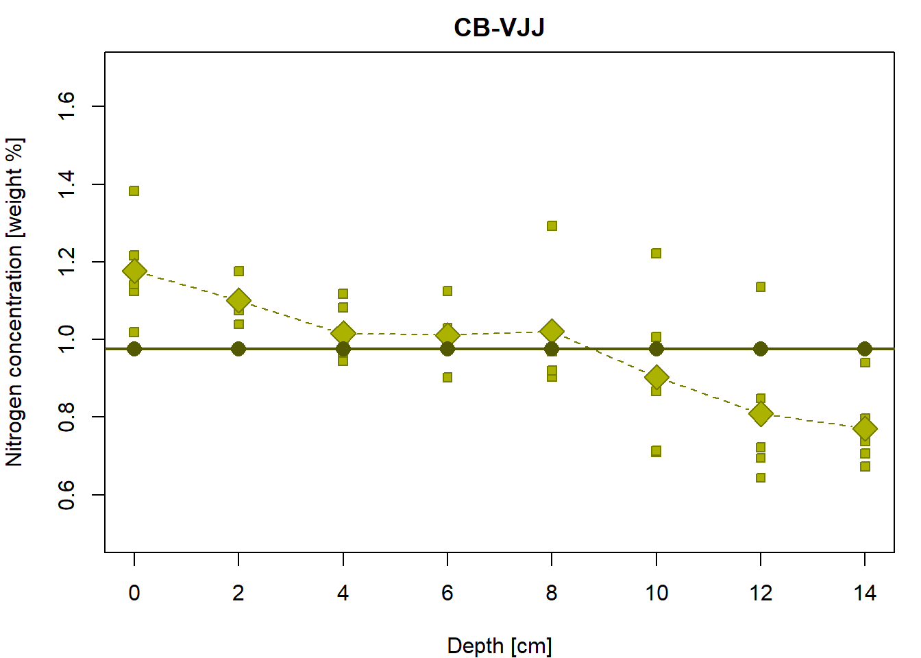
Do you see any relationship with the following?
mean(Yvalues) # beta coefficient## [1] 0.9762055sd(Yvalues) # residual standard error## [1] 0.1827673sd(Yvalues)/sqrt(n) # estimated sd of beta## [1] 0.02889805Total sum of squares:
deviance(fit0) # SST (= RSS of fit0)## [1] 1.302752sum((Yvalues - mean(Yvalues))^2)## [1] 1.302752Overall F-test (once more):
summary(fit1)##
## Call:
## lm(formula = N ~ depth, data = peat, subset = (group == g))
##
## Residuals:
## Min 1Q Median 3Q Max
## -0.19491 -0.09226 -0.01956 0.05038 0.34374
##
## Coefficients:
## Estimate Std. Error t value Pr(>|t|)
## (Intercept) 1.169069 0.038191 30.611 < 2e-16 ***
## depth -0.027552 0.004565 -6.036 5.08e-07 ***
## ---
## Signif. codes: 0 '***' 0.001 '**' 0.01 '*' 0.05 '.' 0.1 ' ' 1
##
## Residual standard error: 0.1323 on 38 degrees of freedom
## Multiple R-squared: 0.4895, Adjusted R-squared: 0.476
## F-statistic: 36.43 on 1 and 38 DF, p-value: 5.083e-07anova(fit0, fit1)## Analysis of Variance Table
##
## Model 1: N ~ 1
## Model 2: N ~ depth
## Res.Df RSS Df Sum of Sq F Pr(>F)
## 1 39 1.3028
## 2 38 0.6651 1 0.63765 36.432 5.083e-07 ***
## ---
## Signif. codes: 0 '***' 0.001 '**' 0.01 '*' 0.05 '.' 0.1 ' ' 1Compare to standard correlation test:
cor.test(Xvalues, Yvalues)##
## Pearson's product-moment correlation
##
## data: Xvalues and Yvalues
## t = -6.0359, df = 38, p-value = 5.083e-07
## alternative hypothesis: true correlation is not equal to 0
## 95 percent confidence interval:
## -0.8301961 -0.4962622
## sample estimates:
## cor
## -0.6996175Depth-as-factor model for the group “CB-VJJ”
Compare fit0 and fit1 with the model where
each depth level is considered separately:
(fit2 = lm(N ~ -1 + as.factor(depth), data = peat, subset = (group == g)))##
## Call:
## lm(formula = N ~ -1 + as.factor(depth), data = peat, subset = (group ==
## g))
##
## Coefficients:
## as.factor(depth)0 as.factor(depth)2 as.factor(depth)4 as.factor(depth)6 as.factor(depth)8
## 1.1769 1.1012 1.0153 1.0114 1.0216
## as.factor(depth)10 as.factor(depth)12 as.factor(depth)14
## 0.9036 0.8086 0.7710par(mfrow = c(1,1), mar = c(4,4,2,1))
# the underlying data
plot(Yvalues ~ Xvalues,pch = PCH[g], col = COL[g], bg = BGC[g],
xlab = XLAB, ylab = YLAB, main = g, xlim = XLIM, ylim = YLIM)
# empirical group means
lines(tabs[[g]][, "Depth"], tabs[[g]][, "Mean"], type="b",
pch = 23, cex = 2, col = COL[g], bg = BGC[g])
# regression line given by the LS estimates (for the specific values of depth)
points(subset(peat, group==g)$depth, fitted(fit2), pch=20, cex=2, col=DARK[g])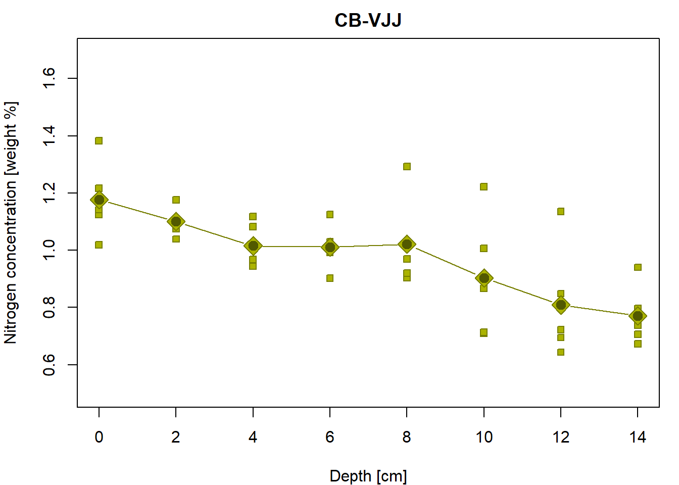
Is it possible to judge (just visually) from the third column whether one assumption of the classical linear model is satisfied? Which assumption?
print(tabs[[g]])## Depth Mean Std.Dev n
## 1 0 1.1769177 0.13512002 5
## 2 2 1.1011507 0.05042430 5
## 3 4 1.0153398 0.07849447 5
## 4 6 1.0113715 0.08000427 5
## 5 8 1.0215852 0.15842290 5
## 6 10 0.9036023 0.21677703 5
## 7 12 0.8086419 0.19742942 5
## 8 14 0.7710349 0.10510728 5Individual work
- Fit lines for every
groupinpeat. - Plot all the fitted lines into one plot, distinguish points and lines by color.
- You can use
jitter()to make the plot even more clear, see below.
Additional material
In some situations (especially if there are lot of data points and no reasonable insight can be made by using a standard plot) a jittered version may be used instead. In this case the depth is randomly shifted by an amount from a uniform distribution on \([-0.5,+0.5]\).
set.seed(123456789)
peat[, "jdepth"] <- peat[, "depth"] + runif(nrow(peat), -0.5, 0.5)
summary(peat)
## group N depth jdepth
## CB :35 Min. :0.4989 Min. : 0.000 Min. :-0.4887
## CB-VJJ:40 1st Qu.:0.8992 1st Qu.: 4.000 1st Qu.: 3.9183
## VJJ :33 Median :1.0343 Median : 8.000 Median : 7.8266
## VJJ-CB:40 Mean :1.0766 Mean : 7.527 Mean : 7.5224
## 3rd Qu.:1.2440 3rd Qu.:12.000 3rd Qu.:11.6579
## Max. :1.6921 Max. :14.000 Max. :14.4483Another plot, this time with the jittered depth:
par(mfrow=c(1,1), mar=c(4,4,0.5,0.5))
plot(N ~ jdepth, data = peat,
     xlab = XLAB, ylab = YLAB, xaxt = "n",
     pch = PCH[group], col = COL[group], bg = BGC[group])
axis(1, at = seq(0, 14, by = 2))
abline(v = seq(1, 13, by = 2), col = "gray", lty = 5, lwd = 2)
legend(1.3, 1.7, legend = levels(peat$group), pch = PCH, col = COL,
       pt.bg = BGC, y.intersp = 1.2)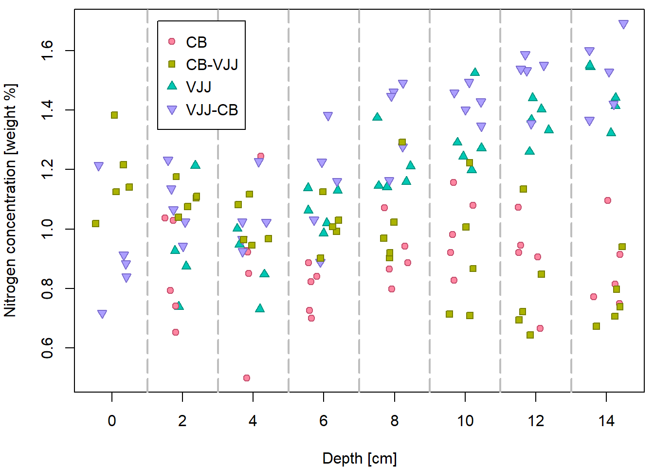
Similar plot using an R function jitter:
par(mfrow=c(1,1), mar=c(4,4,0.5,0.5))
plot(N ~ jitter(depth), data = peat,
     xlab = XLAB, ylab = YLAB,
     pch = PCH[group], col = COL[group], bg = BGC[group])