Model assumptions and graphical diagnostic tools

Download this R markdown as: R, Rmd.

Outline of this lab session:

Model assumptions and diagnostic tools
Graphical diagnostic tools

Loading the data and libraries

Firstly, some necessary R libraries and the working dataset:

library("colorspace")    # colors defined by function
library("mffSM")         # data and plotLM()
library("splines")       # B-splines modelling
library("MASS")          # function stdres for standardized residuals
library("fBasics")       # dagoTest()
library("car")           # ncvTest()
library("lmtest")        # bptest()

We are going to use the dataset Dris from Exercise 6:

data(Dris, package = "mffSM")
# help("Dris")
head(Dris)

##   yield   N  P   K Ca Mg
## 1  5.47 470 47 320 47 11
## 2  5.63 530 48 357 60 16
## 3  5.63 530 48 310 63 16
## 4  4.84 482 47 357 47 13
## 5  4.84 506 48 294 52 15
## 6  4.21 500 45 283 61 14

summary(Dris)

##      yield             N               P               K               Ca              Mg       
##  Min.   :1.920   Min.   :268.0   Min.   :32.00   Min.   :200.0   Min.   :29.00   Min.   : 8.00  
##  1st Qu.:4.040   1st Qu.:427.0   1st Qu.:43.00   1st Qu.:338.0   1st Qu.:41.75   1st Qu.:10.00  
##  Median :4.840   Median :473.0   Median :49.00   Median :377.0   Median :49.00   Median :11.00  
##  Mean   :4.864   Mean   :469.9   Mean   :48.65   Mean   :375.4   Mean   :51.45   Mean   :11.64  
##  3rd Qu.:5.558   3rd Qu.:518.0   3rd Qu.:54.00   3rd Qu.:407.0   3rd Qu.:59.00   3rd Qu.:13.00  
##  Max.   :8.792   Max.   :657.0   Max.   :72.00   Max.   :580.0   Max.   :95.00   Max.   :22.00

par(mar = c(4,4,0.5,0.5))
plot(yield ~ Mg, data  = Dris, lwd=2, col="blue4", bg="skyblue", pch=21)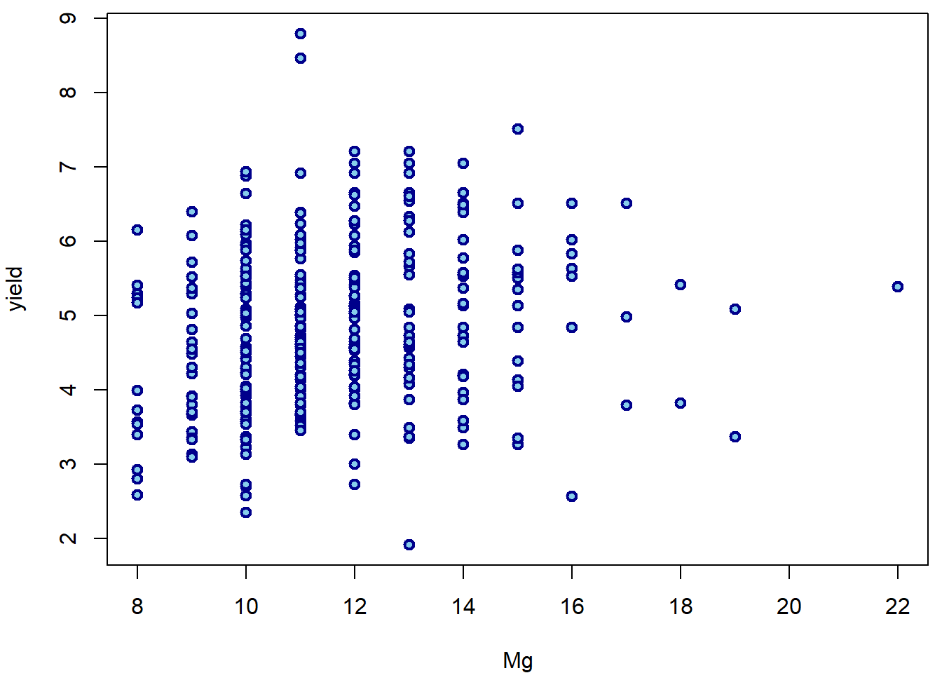

1. Basic model diagnostics

We will use the following model at the beginning:

aLogMg <- lm(yield ~ log2(Mg), data = Dris)
summary(aLogMg)

## 
## Call:
## lm(formula = yield ~ log2(Mg), data = Dris)
## 
## Residuals:
##     Min      1Q  Median      3Q     Max 
## -3.1194 -0.7412 -0.0741  0.7451  3.9841 
## 
## Coefficients:
##             Estimate Std. Error t value Pr(>|t|)    
## (Intercept)   1.4851     0.7790   1.907   0.0574 .  
## log2(Mg)      0.9605     0.2208   4.349 1.77e-05 ***
## ---
## Signif. codes:  0 '***' 0.001 '**' 0.01 '*' 0.05 '.' 0.1 ' ' 1
## 
## Residual standard error: 1.07 on 366 degrees of freedom
## Multiple R-squared:  0.04915,    Adjusted R-squared:  0.04655 
## F-statistic: 18.92 on 1 and 366 DF,  p-value: 1.772e-05

The assumptions on model error terms \(\varepsilon_i\) could be summarized as follows:

independence of the observations,
zero mean, \(\mathsf{E}\, \varepsilon_i = 0, \forall i\),
homoscedasticity, \(\mathsf{var}\, \varepsilon_i = \sigma^2 \forall i\),
normality.

It is only natural to inspect the model residuals to judge whether these assumptions are fulfilled. There are two types of residuals:

Raw residuals \(U_1, \dots, U_n\), that are supposed to satisfy:
- \(\mathsf{E}\, [U_i \mid \boldsymbol{X}_i] = 0\)
- \(\mathsf{var}\, [U_i \mid \boldsymbol{X}_i] = \sigma^2 m_{ii}\), where \(m_{ii}\) is a diagonal element of the matrix \(\mathbb{M} = (\mathbb{I} - \mathbb{H})\)
- in a normal linear model, it also holds that \(U_i\) follow the normal distribution, however, with different variance for different \(i \in \{1, \dots, n\}\)
Standardized residuals \(V_i = U_i / \sqrt{\widehat{\sigma}_n \, m_{ii}} = U_i \sqrt{\frac{n-p}{\mathsf{RSS} \, m_{ii}} }\), for \(i = 1, \dots, n\) that satify
- \(\mathsf{E}\, [V_i \mid \boldsymbol{X}_i] = 0\)
- \(\mathsf{var}\, [V_i \mid \boldsymbol{X}_i] = 1\)
- however, the standardized residuals are not normal – not even under the normal linear model

Here are the three most important nicely formatted graphical diagnostic tools:

par(mar = c(4,4,3,0.5))
plotLM(aLogMg)                # function from 'mffSM'

Individual work

How can we manually reconstruct the plots above?

First plot (Residuals vs Fitted):

par(mfrow = c(1,2), mar = c(4,4,2,0.5))
plot(aLogMg, which = 1)

### manual computation
plot(fitted(aLogMg), residuals(aLogMg),
     lwd=2, col="blue4", bg="skyblue", pch=21)
abline(h=0, col = "grey", lty = 3)
lines(lowess(fitted(aLogMg), residuals(aLogMg)), col="red", lwd=3)
wmaxabs <- order(abs(residuals(aLogMg)), decreasing = TRUE)[1:3]
text(fitted(aLogMg)[wmaxabs], residuals(aLogMg)[wmaxabs], label = wmaxabs, pos = 4)

Second plot (QQ plot):

par(mfrow = c(1,2), mar = c(4,4,2,0.5))
plot(aLogMg, which = 2, ask = FALSE)

### standardized residuals
H = qr.Q(aLogMg[["qr"]]) %*% t(qr.Q(aLogMg[["qr"]]))
M = diag(nrow(H))-H
stdres = residuals(aLogMg)/sqrt(deviance(aLogMg)/aLogMg$df.residual*diag(M))   
qq = qqnorm(stdres, plot.it=FALSE)
# all.equal(stdres(aLogMg), stdres)   # --> TRUE (computed by MASS function)
# all.equal(qq$y, stdres)             # --> TRUE (will be on y-axis)
# all.equal(sort(qq$x), qnorm((1:nrow(Dris)-0.5)/nrow(Dris)))
plot(qq$x, qq$y, lwd=2, col="blue4", bg="skyblue", pch=21)
qqline(stdres, lwd=2, lty=3)
text(qq$x[wmaxabs], qq$y[wmaxabs], label = wmaxabs, pos = ifelse(qq$x[wmaxabs] < 0, 4, 2))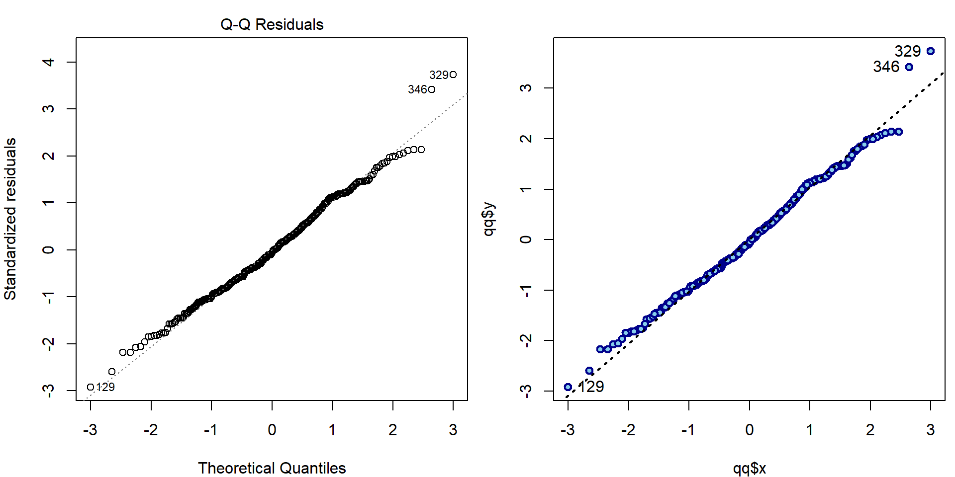

Third plot (Scale-Location plot)

par(mfrow = c(1,2), mar = c(4,4,2,0.5))
plot(aLogMg, which = 3, ask = FALSE)  

### manual computation
plot(fitted(aLogMg), sqrt(abs(stdres)),
     lwd=2, col="blue4", bg="skyblue", pch=21)
lines(lowess(fitted(aLogMg), sqrt(abs(stdres))), col="red", lwd=3)
text(fitted(aLogMg)[wmaxabs], sqrt(abs(stdres))[wmaxabs], label = wmaxabs, pos = 4)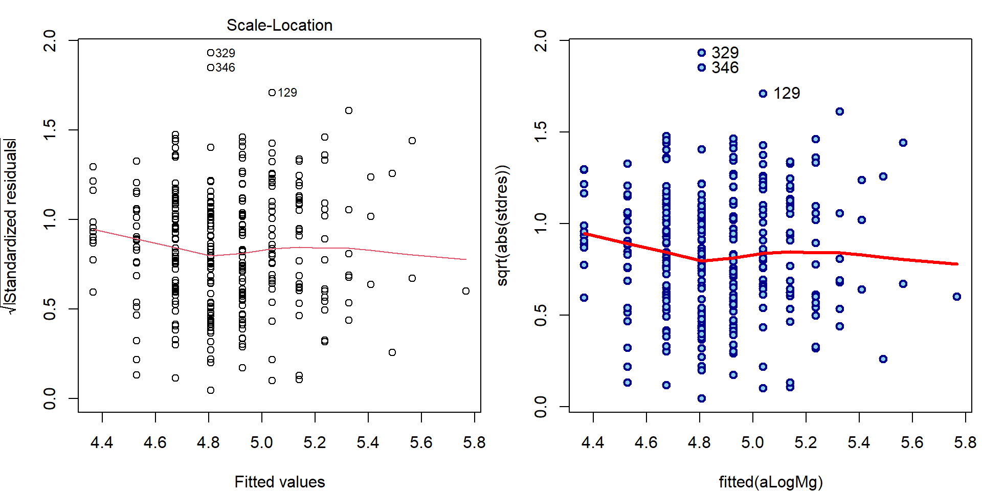

Note, that there are actually infinitely many possibilities how to check that \(\mathsf{E}\,[U_i \mid \boldsymbol{X}_i] = 0\). A scatterplot of fitted values vs. residuals is only one of them. Other common possibility is to plot the covariate values vs. the residuals.

par(mfrow = c(1,2), mar = c(4,4,2,0.5))
plot(log2(Dris$Mg), residuals(aLogMg), 
     xlab=expression(log[2](Mg)), ylab="Residuals", 
     main="Residuals vs. covariate in model", 
     pch = 21, col = "blue4", bg = "skyblue")
lines(lowess(residuals(aLogMg)~log2(Dris$Mg)), col="red")

plot(log2(Dris$Ca), residuals(aLogMg), 
     xlab=expression(log[2](Ca)), ylab="Residuals", 
     main="Residuals vs. covariate not in model", 
     pch = 21, col = "blue4", bg = "skyblue")
lines(lowess(residuals(aLogMg)~log2(Dris$Ca)), col="red")

Also check the following and explain the results:

sum(aLogMg$residuals)

## [1] -5.522666e-14

sum(aLogMg$residuals*log2(Dris$Mg))

## [1] -2.58342e-13

Compare the plots for model aLogMg with the interaction model from previous exercise:

par(mar = c(4,4,3,0.5))
plotLM(lm(yield ~ log2(Mg) + log2(Ca) + I(log2(Mg) * log2(Ca)), data = Dris))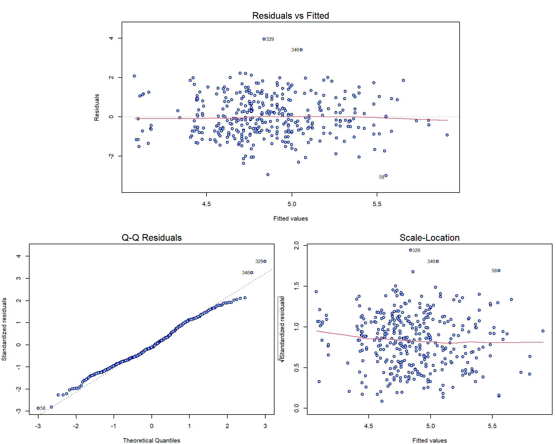

2. Fitting correct \(E[Y \mid \mathbf{X}]\)

The key to make sure \(E[Y \mid \mathbf{X}]\) is fitted correctly is to explore, whether proper parametrizations of covariates are used, which was covered by previous exercises. Here we will demonstrate the necessity of correct parametrization on a data set with extreme behaviour of the response.

A dataset providing a series of (independent) measurements of head acceleration in a simulated motorcycle accident (used to test crash helmets) is given in the datafile Motorcycle (within the R package mffSM).

data(Motorcycle, package = "mffSM")
# help(Motorcycle)
head(Motorcycle)

##   time haccel
## 1  2.4    0.0
## 2  2.6   -1.3
## 3  3.2   -2.7
## 4  3.6    0.0
## 5  4.0   -2.7
## 6  6.2   -2.7

dim(Motorcycle)

## [1] 133   2

summary(Motorcycle)

##       time           haccel       
##  Min.   : 2.40   Min.   :-134.00  
##  1st Qu.:15.80   1st Qu.: -54.90  
##  Median :24.00   Median : -13.30  
##  Mean   :25.55   Mean   : -25.55  
##  3rd Qu.:35.20   3rd Qu.:   0.00  
##  Max.   :65.60   Max.   :  75.00

We are primarily interested in how the head acceleration (covariate haccel) depends on the time after the accident (given in miliseconds – the time covariate).

par(mfrow = c(1,1), mar = c(4,4,1,1))
plot(haccel ~ time, data = Motorcycle, pch = 21, bg = "orange", col = "red3",
     xlab = "Time [ms]", ylab = "Head acceleration [g]")

fit0 = lm(haccel~time, data=Motorcycle)
abline(fit0)

Using the diagnostic plots, we can clearly see that the model denoted as fit0 is hardly appropriate:

par(mar = c(4,4,3,0.5))
plotLM(fit0)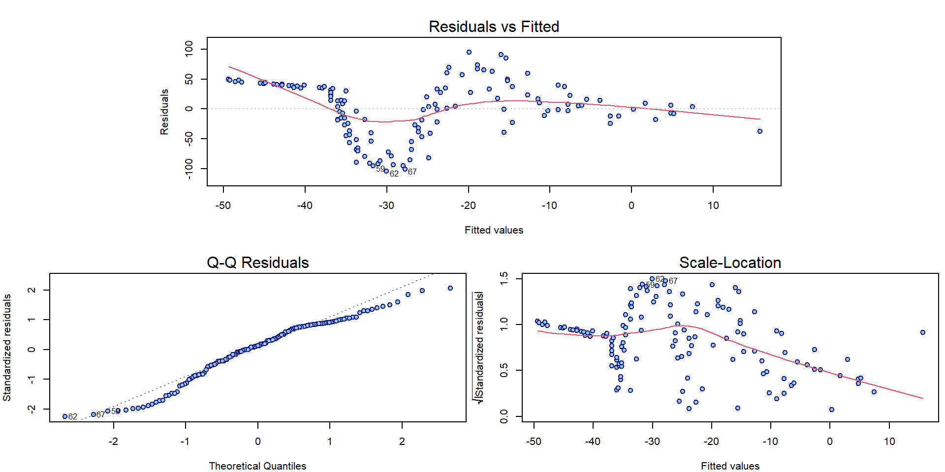

As far as there is a quite flexible shape observed in the plot we need some more flexible model to capture the structure of the underlying conditional expectation of the head acceleration given the time.

Polynomials and splines

We will use polynomials (of different degrees) for fitting the model (while still staying within the linear regression framework).

fit6 <- lm(haccel~poly(time, 6, raw=TRUE), data=Motorcycle)  
fit12 <- lm(haccel~poly(time, 12, raw=TRUE), data=Motorcycle)

The model can be visualized as follows:

xgrid <- seq(0, 70, length = 500)

par(mfrow = c(1,1), mar = c(4,4,2,1))
plot(haccel ~ time, data = Motorcycle, pch = 21, bg = "orange", col = "red3",
     main = "Fitted polynomial curves",
     xlab = "Time [ms]", ylab = "Head acceleration [g]")
lines(xgrid, predict(fit6, newdata=data.frame(time=xgrid)), lwd=2, col="blue")
lines(xgrid, predict(fit12, newdata=data.frame(time=xgrid)), lwd=2, col="darkgreen")
legend(37,-70, lty=rep(1, 2), col=c("blue", "darkgreen"), 
       legend=paste("p=", c(6,12),sep=""), lwd=c(2,2), cex=1.2)

Classical polynomials are, however, not computationally very effective. Especially for higher order of the polynomial approximation the solution tends to be unstable. To avoid numerical problems you can use orthogonal polynomials with raw=FALSE, which stabilizes the magnitude (and standard errors) of estimated coefficients:

summary(fit6)

## 
## Call:
## lm(formula = haccel ~ poly(time, 6, raw = TRUE), data = Motorcycle)
## 
## Residuals:
##     Min      1Q  Median      3Q     Max 
## -76.039 -23.622  -0.497  24.032  75.521 
## 
## Coefficients:
##                              Estimate Std. Error t value Pr(>|t|)    
## (Intercept)                -2.069e+02  4.349e+01  -4.757 5.29e-06 ***
## poly(time, 6, raw = TRUE)1  9.658e+01  1.558e+01   6.199 7.47e-09 ***
## poly(time, 6, raw = TRUE)2 -1.302e+01  1.865e+00  -6.982 1.49e-10 ***
## poly(time, 6, raw = TRUE)3  7.160e-01  1.012e-01   7.078 9.04e-11 ***
## poly(time, 6, raw = TRUE)4 -1.870e-02  2.732e-03  -6.846 2.97e-10 ***
## poly(time, 6, raw = TRUE)5  2.321e-04  3.572e-05   6.496 1.73e-09 ***
## poly(time, 6, raw = TRUE)6 -1.102e-06  1.799e-07  -6.128 1.05e-08 ***
## ---
## Signif. codes:  0 '***' 0.001 '**' 0.01 '*' 0.05 '.' 0.1 ' ' 1
## 
## Residual standard error: 33.09 on 126 degrees of freedom
## Multiple R-squared:  0.5524, Adjusted R-squared:  0.5311 
## F-statistic: 25.91 on 6 and 126 DF,  p-value: < 2.2e-16

summary(lm(haccel~poly(time, 6, raw=FALSE), data=Motorcycle))

## 
## Call:
## lm(formula = haccel ~ poly(time, 6, raw = FALSE), data = Motorcycle)
## 
## Residuals:
##     Min      1Q  Median      3Q     Max 
## -76.039 -23.622  -0.497  24.032  75.521 
## 
## Coefficients:
##                             Estimate Std. Error t value Pr(>|t|)    
## (Intercept)                  -25.546      2.869  -8.903 5.01e-15 ***
## poly(time, 6, raw = FALSE)1  160.611     33.091   4.854 3.52e-06 ***
## poly(time, 6, raw = FALSE)2   99.015     33.091   2.992  0.00333 ** 
## poly(time, 6, raw = FALSE)3 -244.969     33.091  -7.403 1.67e-11 ***
## poly(time, 6, raw = FALSE)4   64.683     33.091   1.955  0.05283 .  
## poly(time, 6, raw = FALSE)5  171.291     33.091   5.176 8.68e-07 ***
## poly(time, 6, raw = FALSE)6 -202.776     33.091  -6.128 1.05e-08 ***
## ---
## Signif. codes:  0 '***' 0.001 '**' 0.01 '*' 0.05 '.' 0.1 ' ' 1
## 
## Residual standard error: 33.09 on 126 degrees of freedom
## Multiple R-squared:  0.5524, Adjusted R-squared:  0.5311 
## F-statistic: 25.91 on 6 and 126 DF,  p-value: < 2.2e-16

Another possible solution how to introduce some reasonable stability into the model where some higher order polynomials are used, are splines.

### Choice of knots 
knots <- c(0, 11, 12, 13, 20, 30, 32, 34, 40, 50, 70) 
(inner <- knots[-c(1, length(knots))])  # inner knots

## [1] 11 12 13 20 30 32 34 40 50

(bound <- knots[c(1, length(knots))])   # boundary knots

## [1]  0 70

### B-splines of degree 3
DEGREE <- 3 # piecewise cubic 
Bgrid <- bs(xgrid, knots = inner, Boundary.knots = bound, degree = DEGREE, 
            intercept = TRUE)
dim(Bgrid)   # 13-dimensional linear space of piecewise polynomials

## [1] 500  13

The B-spline basis is a set of the following functions:

COL <- rainbow_hcl(ncol(Bgrid), c = 80)
par(mfrow = c(1,1), mar = c(4,4,1,1))
plot(xgrid, Bgrid[,1], type = "l", col = COL[1], lwd = 2, xlab = "x", 
     ylab = "B(x)", xlim = range(knots), ylim = range(Bgrid, na.rm = TRUE))
for (j in 2:ncol(Bgrid)) lines(xgrid, Bgrid[,j], col = COL[j], lwd = 2)
points(knots, rep(0, length(knots)), 
       pch = 21, bg = "blue", col = "skyblue", cex = 1.5)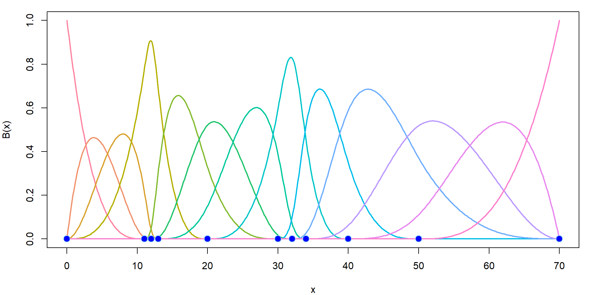

Thus, we can use B-splines to fit the model.

More details about the B-splines can be found, for instance, here.

m1 <- lm(haccel ~ bs(time, knots = inner, Boundary.knots = bound, 
                     degree = DEGREE, intercept = TRUE) - 1, data = Motorcycle)

This is the fitted curve:

par(mfrow = c(1,1), mar = c(4,4,2,1))
plot(haccel ~ time, data = Motorcycle, pch = 21, bg = "orange", col = "red3",
     main = "Fitted B-spline curve",
     xlab = "Time [ms]", ylab = "Head acceleration [g]")
lines(xgrid, predict(m1, newdata=data.frame(time=xgrid)), lwd=2, col="blue")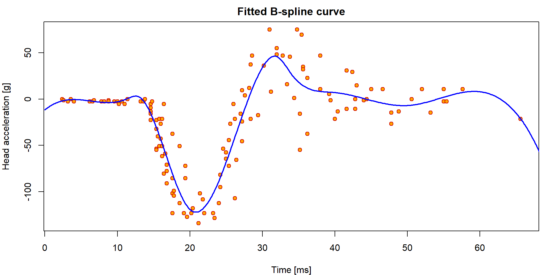

names(m1$coefficients) <- paste("B", 1:ncol(Bgrid))
summary(m1)

## 
## Call:
## lm(formula = haccel ~ bs(time, knots = inner, Boundary.knots = bound, 
##     degree = DEGREE, intercept = TRUE) - 1, data = Motorcycle)
## 
## Residuals:
##     Min      1Q  Median      3Q     Max 
## -71.857 -11.740  -0.268  10.356  55.249 
## 
## Coefficients:
##      Estimate Std. Error t value Pr(>|t|)    
## B 1   -11.614     83.252  -0.140    0.889    
## B 2    12.450     81.282   0.153    0.879    
## B 3   -13.988     45.345  -0.308    0.758    
## B 4     2.984     18.894   0.158    0.875    
## B 5     6.115     12.139   0.504    0.615    
## B 6  -237.283     18.850 -12.588  < 2e-16 ***
## B 7    17.346     14.094   1.231    0.221    
## B 8    53.248     12.635   4.214 4.88e-05 ***
## B 9     5.102     13.051   0.391    0.697    
## B 10   12.609     17.146   0.735    0.464    
## B 11  -34.949     38.161  -0.916    0.362    
## B 12   58.255     65.045   0.896    0.372    
## B 13  -93.068     75.924  -1.226    0.223    
## ---
## Signif. codes:  0 '***' 0.001 '**' 0.01 '*' 0.05 '.' 0.1 ' ' 1
## 
## Residual standard error: 22.61 on 120 degrees of freedom
## Multiple R-squared:  0.8447, Adjusted R-squared:  0.8278 
## F-statistic: 50.19 on 13 and 120 DF,  p-value: < 2.2e-16

Since the intercept is included within the B-spline basis (intercept = TRUE in bs), we omitted it in the formula with -1. However, this use comes with some issues deeply rooted within the implementation. For example, neither Multiple R-squared nor the F-statistic quantity in the output correspond to correct numbers. Simply put, summary.lm thinks the intercept is not included despite still being a linear combination of given columns.

Individual work

Can you explain why the values reported for \(R^2\) and \(R_{adj}^2\) are not appropriate? What is the right meaning of these numbers? Can you manually reconstruct them?

The \(R^2\) value from the model is

summary(m1)$r.squared

## [1] 0.8446597

and the manual calculations will give

1 - deviance(m1)/sum(Motorcycle$haccel^2)

## [1] 0.8446597

sum(fitted(m1)^2)/sum(Motorcycle$haccel^2)

## [1] 0.8446597

Interpretation of the F-test from the summary output above is a test of a submodel

summary(m1)$fstatistic

##     value     numdf     dendf 
##  50.19211  13.00000 120.00000

# the usual F-test (correct)
m2 <- lm(haccel ~ 1, data = Motorcycle)
anova(m2, m1)

## Analysis of Variance Table
## 
## Model 1: haccel ~ 1
## Model 2: haccel ~ bs(time, knots = inner, Boundary.knots = bound, degree = DEGREE, 
##     intercept = TRUE) - 1
##   Res.Df    RSS Df Sum of Sq     F    Pr(>F)    
## 1    132 308223                                 
## 2    120  61362 12    246861 40.23 < 2.2e-16 ***
## ---
## Signif. codes:  0 '***' 0.001 '**' 0.01 '*' 0.05 '.' 0.1 ' ' 1

# the wrong F-test (in summary m1)
(m0 <- lm(haccel ~ -1, data=Motorcycle))

## 
## Call:
## lm(formula = haccel ~ -1, data = Motorcycle)
## 
## No coefficients

anova(m0 ,m1)

## Analysis of Variance Table
## 
## Model 1: haccel ~ -1
## Model 2: haccel ~ bs(time, knots = inner, Boundary.knots = bound, degree = DEGREE, 
##     intercept = TRUE) - 1
##   Res.Df    RSS Df Sum of Sq      F    Pr(>F)    
## 1    133 395017                                  
## 2    120  61362 13    333655 50.192 < 2.2e-16 ***
## ---
## Signif. codes:  0 '***' 0.001 '**' 0.01 '*' 0.05 '.' 0.1 ' ' 1

Nevertheless, as the intercept parameter is in the linear span of the columns of \(\mathbb{X}\), it makes sense to calculate the (usual) multiple \(R^2\) value. This can be done ‘manually’ as follows:

var(fitted(m1)) / var(Motorcycle$haccel)

## [1] 0.8009163

cor(Motorcycle$haccel, fitted(m1))^2

## [1] 0.8009163

1 - deviance(m1)/deviance(m2)

## [1] 0.8009163

Alternatively, one can use B-splines (the basis without intercept) with an intercept in the model to get some meaningful numbers in the output:

m3 <- lm(haccel ~ bs(time, knots = inner, Boundary.knots = bound, 
                     degree = DEGREE, intercept = FALSE), data = Motorcycle)
names(m3$coefficients) <- c("(Intercept)", paste("B", 1:12))
summary(m3)

## 
## Call:
## lm(formula = haccel ~ bs(time, knots = inner, Boundary.knots = bound, 
##     degree = DEGREE, intercept = FALSE), data = Motorcycle)
## 
## Residuals:
##     Min      1Q  Median      3Q     Max 
## -71.857 -11.740  -0.268  10.356  55.249 
## 
## Coefficients:
##             Estimate Std. Error t value Pr(>|t|)  
## (Intercept)  -11.614     83.252  -0.140   0.8893  
## B 1           24.064    161.970   0.149   0.8821  
## B 2           -2.374     57.835  -0.041   0.9673  
## B 3           14.598     93.327   0.156   0.8760  
## B 4           17.729     80.496   0.220   0.8261  
## B 5         -225.669     88.698  -2.544   0.0122 *
## B 6           28.960     82.780   0.350   0.7271  
## B 7           64.862     84.773   0.765   0.4457  
## B 8           16.716     83.997   0.199   0.8426  
## B 9           24.223     85.172   0.284   0.7766  
## B 10         -23.335     91.337  -0.255   0.7988  
## B 11          69.869    105.918   0.660   0.5107  
## B 12         -81.454    112.465  -0.724   0.4703  
## ---
## Signif. codes:  0 '***' 0.001 '**' 0.01 '*' 0.05 '.' 0.1 ' ' 1
## 
## Residual standard error: 22.61 on 120 degrees of freedom
## Multiple R-squared:  0.8009, Adjusted R-squared:  0.781 
## F-statistic: 40.23 on 12 and 120 DF,  p-value: < 2.2e-16

anova(m2,m3)

## Analysis of Variance Table
## 
## Model 1: haccel ~ 1
## Model 2: haccel ~ bs(time, knots = inner, Boundary.knots = bound, degree = DEGREE, 
##     intercept = FALSE)
##   Res.Df    RSS Df Sum of Sq     F    Pr(>F)    
## 1    132 308223                                 
## 2    120  61362 12    246861 40.23 < 2.2e-16 ***
## ---
## Signif. codes:  0 '***' 0.001 '**' 0.01 '*' 0.05 '.' 0.1 ' ' 1

What about the interpretation of the classical diagnostic plots for the model fitted with B-splines?

par(mar = c(4,4,3,0.5))
plotLM(m1)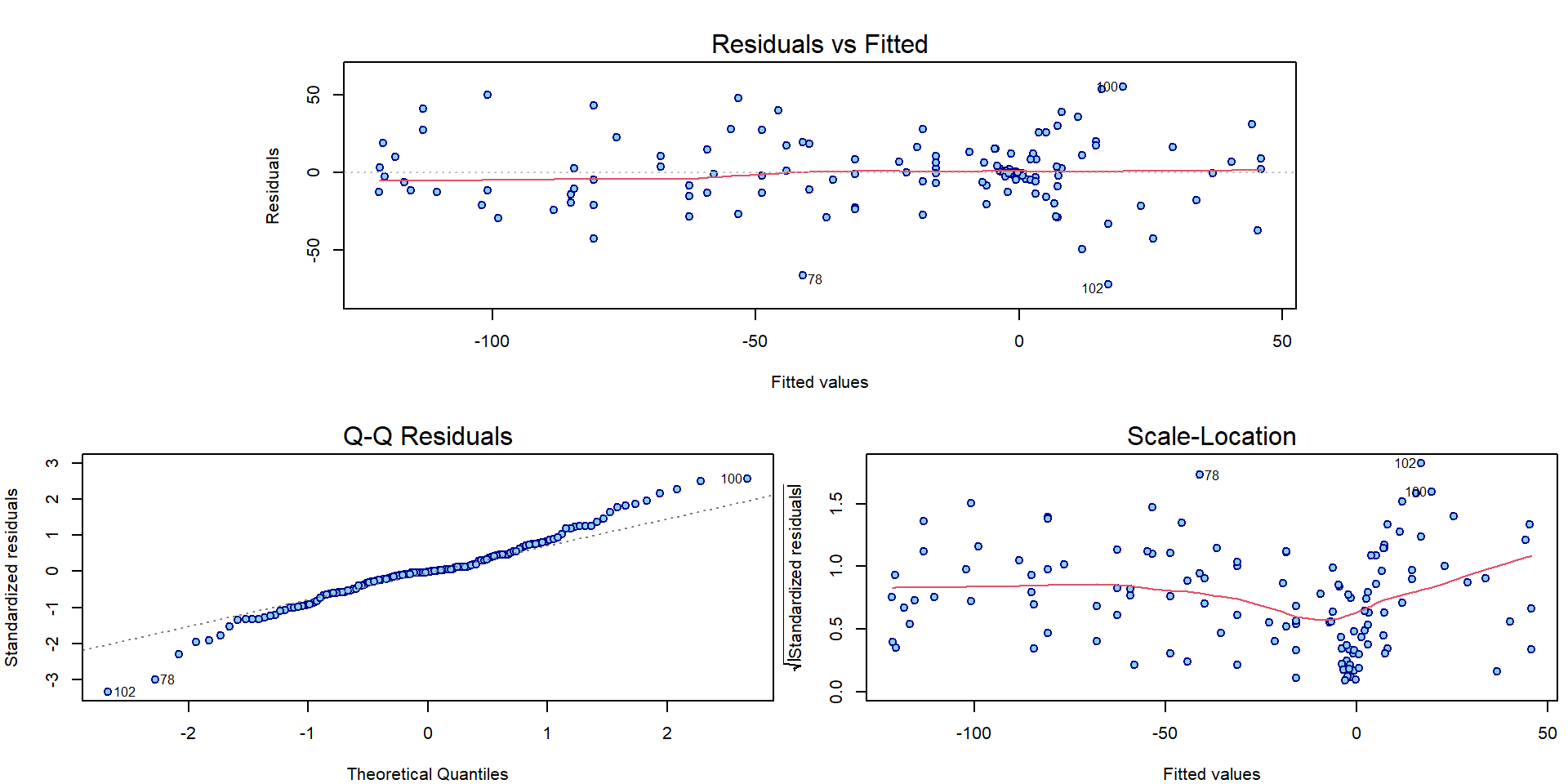

It seems there is some issue with homoscedasticity assumption. Let’s change the x-axis of the third Scale-Location plot to determine how the variability changes:

par(mfrow = c(1,2), mar = c(4,4,2,1))
plot(abs(fitted(m1)), sqrt(abs(stdres(m1))),
     main = "Abs(fitted)",
     lwd=2, col="blue4", bg="skyblue", pch=21)
lines(lowess(abs(fitted(m1)), sqrt(abs(stdres(m1)))), col="red", lwd=3)

plot(Motorcycle$time, sqrt(abs(stdres(m1))),
     main = "Time",
     lwd=2, col="blue4", bg="skyblue", pch=21)
lines(lowess(Motorcycle$time, sqrt(abs(stdres(m1)))), col="red", lwd=3)

How to adjust the inference for heteroscedastic models will be shown next exercise.

3. Log transformation of the response

We will use a small dataset (47 observations and 8 different covariates) containing some pieces of information about fires that occurred in Chicago in 1970 while distinguishing for some information provided in the data. Particularly, we will focus on the locality in Chicago (north vs. south) and the proportion of minority citizens. The dataset is loaded from the website and some brief insight is provided below.

chicago <- read.csv("http://www.karlin.mff.cuni.cz/~vavraj/nmfm334/data/chicago.csv", 
                    header=T, stringsAsFactors = TRUE)
        
chicago <- transform(chicago, 
                     fside = factor(side, levels = 0:1, labels=c("North", "South")))          
                    
head(chicago)

##   minor fire theft  old insur income side fside
## 1  10.0  6.2    29 60.4   0.0 11.744    0 North
## 2  22.2  9.5    44 76.5   0.1  9.323    0 North
## 3  19.6 10.5    36 73.5   1.2  9.948    0 North
## 4  17.3  7.7    37 66.9   0.5 10.656    0 North
## 5  24.5  8.6    53 81.4   0.7  9.730    0 North
## 6  54.0 34.1    68 52.6   0.3  8.231    0 North

summary(chicago)

##      minor            fire           theft             old            insur            income      
##  Min.   : 1.00   Min.   : 2.00   Min.   :  3.00   Min.   : 2.00   Min.   :0.0000   Min.   : 5.583  
##  1st Qu.: 3.75   1st Qu.: 5.65   1st Qu.: 22.00   1st Qu.:48.60   1st Qu.:0.0000   1st Qu.: 8.447  
##  Median :24.50   Median :10.40   Median : 29.00   Median :65.00   Median :0.4000   Median :10.694  
##  Mean   :34.99   Mean   :12.28   Mean   : 32.36   Mean   :60.33   Mean   :0.6149   Mean   :10.696  
##  3rd Qu.:57.65   3rd Qu.:16.05   3rd Qu.: 38.00   3rd Qu.:77.30   3rd Qu.:0.9000   3rd Qu.:11.989  
##  Max.   :99.70   Max.   :39.70   Max.   :147.00   Max.   :90.10   Max.   :2.2000   Max.   :21.480  
##       side          fside   
##  Min.   :0.0000   North:25  
##  1st Qu.:0.0000   South:22  
##  Median :0.0000             
##  Mean   :0.4681             
##  3rd Qu.:1.0000             
##  Max.   :1.0000

The data contain information from Chicago insurance redlining in 47 districts in 1970 where

minor stands for the percentage of minority (0 - 100) in a given district,
fire stands for the number of fires per 100 households during the reference period,
theft denotes the number of reported thefts per 1000 inhabitants,
old gives percentage of residential units built before 1939,
insur states the number of policies per 100 household,
income is the median income (USD 1000) per household,
side gives the location of the district within Chicago (0 = North, 1 = South).

Exploration

We wish to describe the dependence of the number of fires (fire) on the percentage of minority (minor). We are also aware of the fact that the form of this dependence may differ in north and south parts of Chicago.

par(mfrow = c(1,1), mar = c(4,4,0.5,0.5))
XLAB <- "Minority (%)"
YLAB <- "Fires (#/100 households)"
COLS <- c(North = "darkgreen", South = "red")
BGS <- c(North = "aquamarine", South = "orange")
PCHS <- c(North = 21, South = 23)
plot(fire ~ minor, data = chicago, 
     xlab = XLAB, ylab = YLAB, 
     col = COLS[fside], bg = BGS[fside], pch = PCHS[fside])
legend("topleft", legend = c("North", "South"), bty = "n", 
       pch = PCHS, col = COLS, pt.bg = BGS)
lines(with(subset(chicago, fside == "North"), lowess(minor, fire)),
      col = COLS["North"], lwd = 2)
lines(with(subset(chicago, fside == "South"), lowess(minor, fire)), 
      col = COLS["South"], lwd = 2)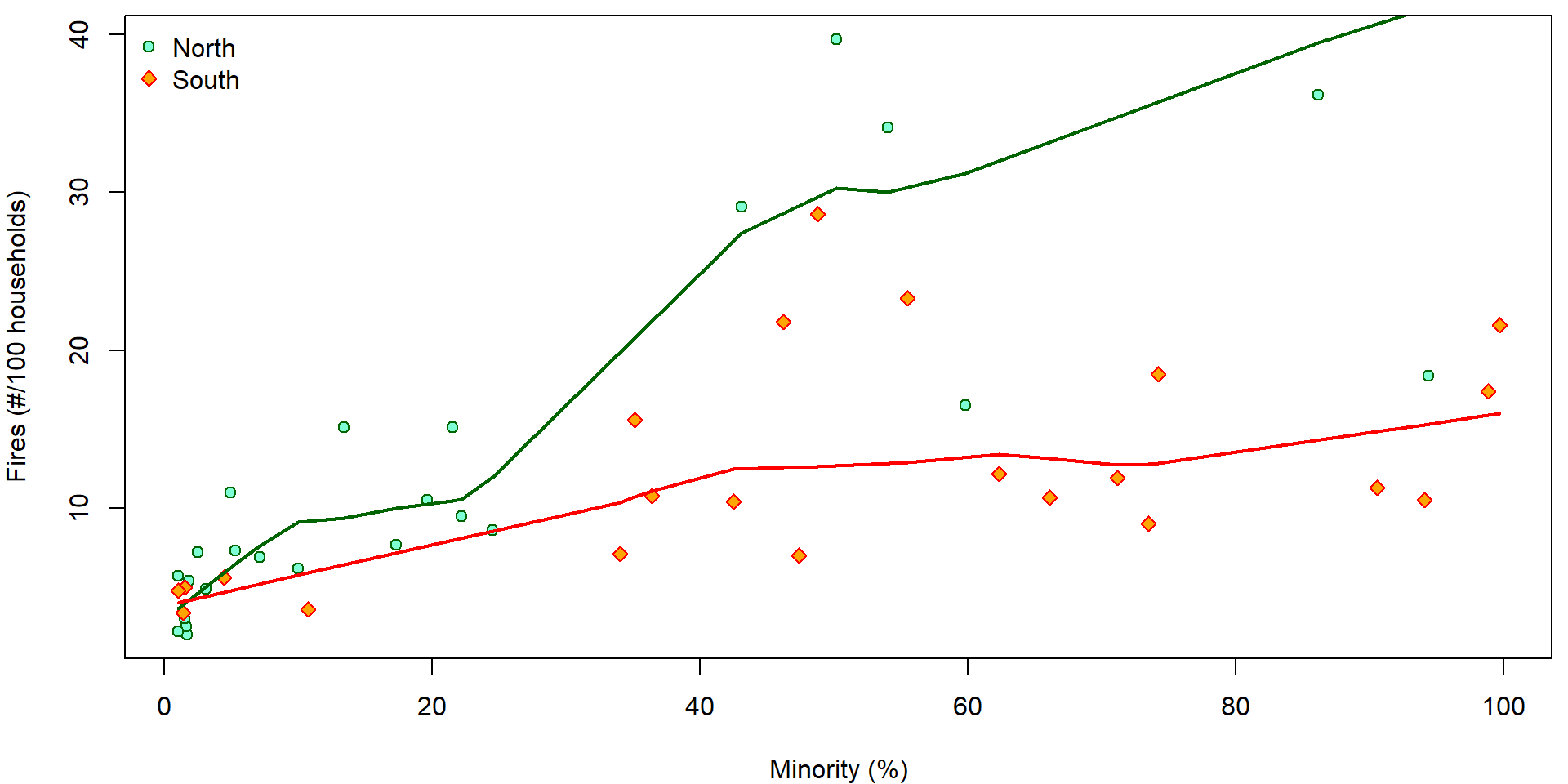

Lets fit different lines for the two sides of Chicago.

mlines <- lm(fire ~ minor * fside, data = chicago)
summary(mlines)

## 
## Call:
## lm(formula = fire ~ minor * fside, data = chicago)
## 
## Residuals:
##     Min      1Q  Median      3Q     Max 
## -17.262  -3.340  -1.474   3.075  18.303 
## 
## Coefficients:
##                  Estimate Std. Error t value Pr(>|t|)    
## (Intercept)       5.19515    1.69212   3.070   0.0037 ** 
## minor             0.32274    0.04896   6.592 5.03e-08 ***
## fsideSouth        1.37454    3.10252   0.443   0.6600    
## minor:fsideSouth -0.20812    0.06589  -3.159   0.0029 ** 
## ---
## Signif. codes:  0 '***' 0.001 '**' 0.01 '*' 0.05 '.' 0.1 ' ' 1
## 
## Residual standard error: 6.535 on 43 degrees of freedom
## Multiple R-squared:  0.5387, Adjusted R-squared:  0.5065 
## F-statistic: 16.74 on 3 and 43 DF,  p-value: 2.376e-07

And create the corresponding diagnostic plots:

par(mar = c(4,4,2,0.5))
plotLM(mlines)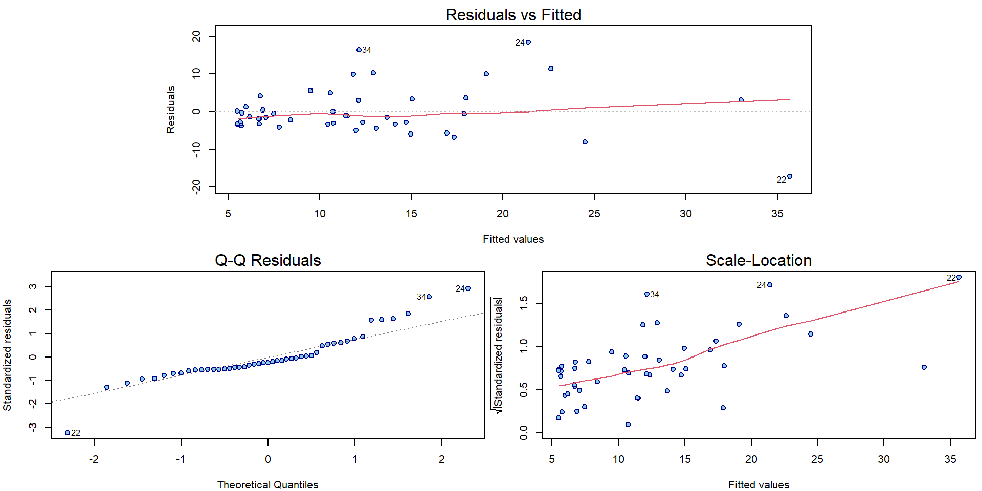

We observe some issues with normality assumption, but especially large issues with increasing variability.

Some statistical tests for normality applied to residuals that are heteroscedastic (even in homoscedastic model):

shapiro.test(residuals(mlines))

## 
##  Shapiro-Wilk normality test
## 
## data:  residuals(mlines)
## W = 0.90361, p-value = 0.0009409

dagoTest(residuals(mlines))

## 
## Title:
##  D'Agostino Normality Test
## 
## Test Results:
##   STATISTIC:
##     Chi2 | Omnibus: 9.4764
##     Z3  | Skewness: 2.1817
##     Z4  | Kurtosis: 2.1717
##   P VALUE:
##     Omnibus  Test: 0.008754 
##     Skewness Test: 0.02913 
##     Kurtosis Test: 0.02987

Some statistical tests for normality applied to standardized residuals that are not normal (even in normal linear model):

shapiro.test(stdres(mlines))

## 
##  Shapiro-Wilk normality test
## 
## data:  stdres(mlines)
## W = 0.90005, p-value = 0.0007228

dagoTest(stdres(mlines))

## 
## Title:
##  D'Agostino Normality Test
## 
## Test Results:
##   STATISTIC:
##     Chi2 | Omnibus: 7.9183
##     Z3  | Skewness: 1.3467
##     Z4  | Kurtosis: 2.4707
##   P VALUE:
##     Omnibus  Test: 0.01908 
##     Skewness Test: 0.1781 
##     Kurtosis Test: 0.01348

Statistical test for homoscedasticity (Breusch-Pagan test and Koenker’s studentized version) with alternatives \(\mathsf{var} \left[ Y_i | \mathbf{X}_i\right] = \sigma^2 \exp\left\{\tau \mathsf{E} \left[Y_i | \mathbf{X}_i\right]\right\}\) or in general \(\mathsf{var} \left[ Y_i | \mathbf{X}_i, \mathbf{Z_i}\right] = \sigma^2 \exp\left\{\mathbf{Z}_i^\top \boldsymbol{\tau}\right\}\):

ncvTest(mlines)                                     # default is fitted

## Non-constant Variance Score Test 
## Variance formula: ~ fitted.values 
## Chisquare = 25.2439, Df = 1, p = 5.0519e-07

ncvTest(mlines, var.formula = ~fitted(mlines))      # the same as before

## Non-constant Variance Score Test 
## Variance formula: ~ fitted(mlines) 
## Chisquare = 25.2439, Df = 1, p = 5.0519e-07

bptest(mlines, varformula = ~fitted(mlines))        # Koenker's studentized version (robust to non-normality)

## 
##  studentized Breusch-Pagan test
## 
## data:  mlines
## BP = 13.692, df = 1, p-value = 0.0002153

bptest(mlines)                                      # default is the same as model formula

## 
##  studentized Breusch-Pagan test
## 
## data:  mlines
## BP = 15.212, df = 3, p-value = 0.001644

In addition, there is also a bunch of points scattered around the origin and relatively only a few observations are given for larger proportion of the minority or the larger amount of fires. This suggests that log transformation (of the response and the predictor as well) could help.

Interpretation of a model with log-transformed response

Typically, when the residual variance increases with the response expectation, log-transformation of the response often ensures a homoscedastic model (Assumption A3a from the lecture).

Firstly, compare the plot below (on the log scale on \(y\) axes) with the previous plot on the original scale on the \(y\) axes:

par(mfrow = c(1,1), mar = c(4,4,0.5,0.5))
LYLAB <- "Log(Fires)"
plot(log(fire) ~ minor, data = chicago, 
     xlab = XLAB, ylab = LYLAB, 
     col = COLS[fside], bg = BGS[fside], pch = PCHS[fside])
legend("topleft", legend = c("North", "South"), bty = "n", 
       pch = PCHS,  col = COLS, pt.bg = BGS)
lines(with(subset(chicago, fside == "North"), lowess(minor, log(fire))), 
      col = COLS["North"], lwd = 2)
lines(with(subset(chicago, fside == "South"), lowess(minor, log(fire))), 
      col = COLS["South"], lwd = 2)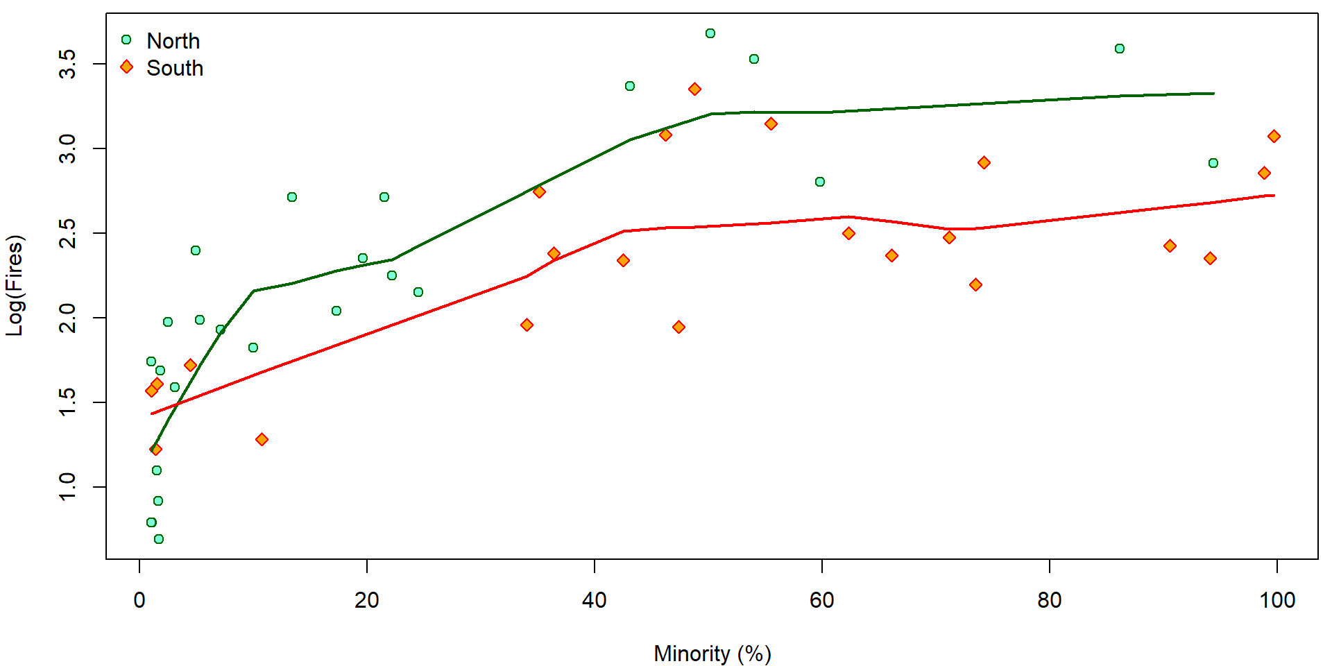

Using the proposed transformation of the response we also change the underlying data. This means, that instead of the model \[ \mathsf{E} [Y_i | \boldsymbol{X}_i] = \boldsymbol{X}_i^\top \boldsymbol{\beta} \] fitted based on the random sample \(\{(Y_i, \boldsymbol{X}_i);\; i = 1, \dots, n\}\) we fit another model of the form \[ \mathsf{E} [\log(Y_i) | \boldsymbol{X}_i] = \boldsymbol{X}_i^\top \widetilde{\boldsymbol{\beta}} \] which is, however, based on the different random sample \(\{(\log(Y_i), \boldsymbol{X}_i);\;i = 1, \dots, n\}\). This has some crucial consequences. The logarithmic transformation will help to deal with some issues regarding heteroscedastic data but, on the other hand, it will introduce new problems regarding the model interpretability.

The idea is that the final model should be (always) interpreted with respect to the original data - the information about the number of fires (fire) - not the logarithm of the number of fires (log(fire)).

For some better interpretation we will also use the log transformation of the independent variable – the information about the proportion of minority – minor. What is the interpretation of the following model:

summary(m <- lm(log(fire) ~ log2(minor) * fside, data = chicago))

## 
## Call:
## lm(formula = log(fire) ~ log2(minor) * fside, data = chicago)
## 
## Residuals:
##      Min       1Q   Median       3Q      Max 
## -0.75178 -0.33949 -0.07901  0.34564  0.84890 
## 
## Coefficients:
##                        Estimate Std. Error t value Pr(>|t|)    
## (Intercept)             1.01616    0.14635   6.943 1.55e-08 ***
## log2(minor)             0.35961    0.03853   9.332 6.74e-12 ***
## fsideSouth              0.27963    0.26983   1.036   0.3058    
## log2(minor):fsideSouth -0.14411    0.05772  -2.497   0.0164 *  
## ---
## Signif. codes:  0 '***' 0.001 '**' 0.01 '*' 0.05 '.' 0.1 ' ' 1
## 
## Residual standard error: 0.4149 on 43 degrees of freedom
## Multiple R-squared:  0.7278, Adjusted R-squared:  0.7088 
## F-statistic: 38.33 on 3 and 43 DF,  p-value: 3.234e-12

The diagnostic plots have improved in terms of mean and variance:

par(mar = c(4,4,2,0.5))
plotLM(m)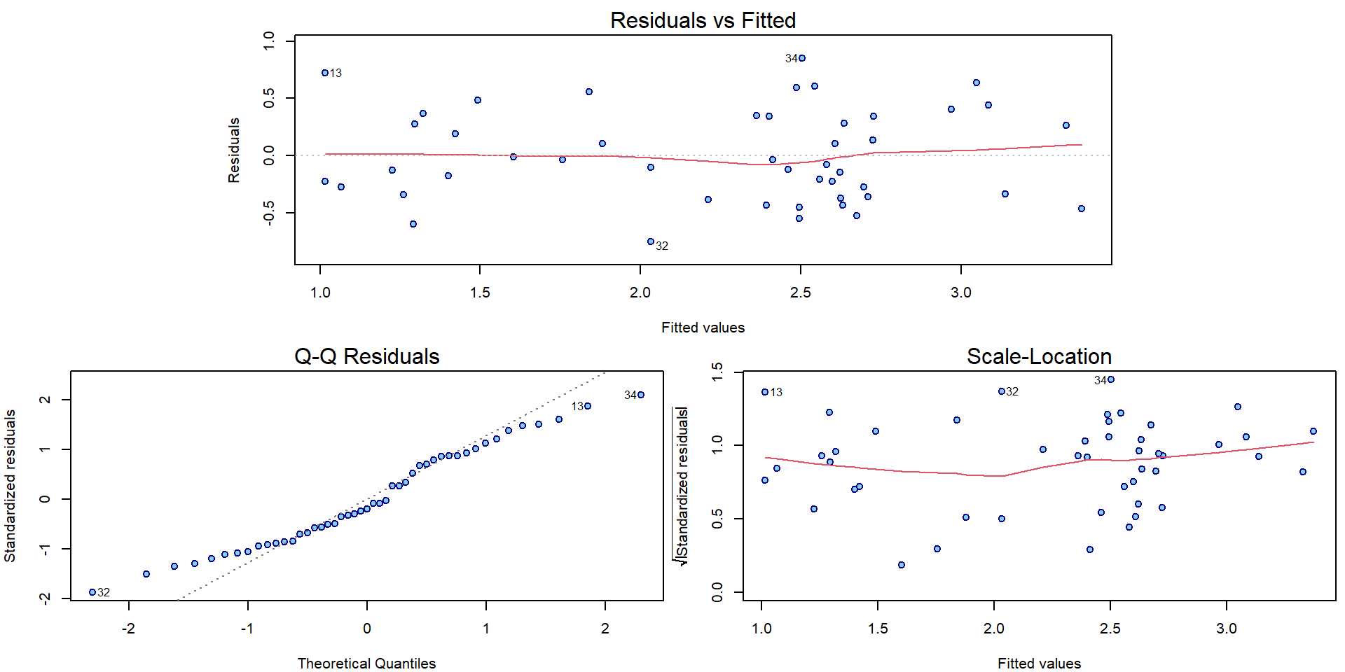

Recall the Jensen inequality and the fact that \[ \mathsf{E} [\log(Y_i) | \boldsymbol{X}_i] \neq \log(\mathsf{E} [Y_i | \boldsymbol{X}_i]) \qquad \text{but rather} \qquad \mathsf{E} [\log(Y_i) | \boldsymbol{X}_i] < \log(\mathsf{E} [Y_i | \boldsymbol{X}_i]). \] And now compare the two models: \[ \begin{aligned} Y_i &= \mathbf{X}_i^\top \boldsymbol{\beta} + \varepsilon_i, \\ \log Y_i = \mathbf{X}_i^\top \widetilde{\boldsymbol{\beta}} + \widetilde{\varepsilon}_i \quad\Longleftrightarrow\quad Y_i &= \exp\left\{\mathbf{X}_i^\top \widetilde{\boldsymbol{\beta}}\right\} \cdot \exp\left\{ \widetilde{\varepsilon}_i \right\}. \end{aligned} \]

What are the consequences with respect to the interpretation of the parameter estimates provided in the summary output above? What would be a suitable interpretation that we can use in this situation?

\[ \dfrac{ \mathsf{E} \left[Y_i | \mathbf{X}_i = \mathbf{x} + \mathbf{e}_j\right] }{ \mathsf{E} \left[Y_i | \mathbf{X}_i = \mathbf{x}\right] } = \dfrac{ \exp \left\{ (\mathbf{x} + \mathbf{e}_j)^\top \widetilde{\boldsymbol{\beta}} \right\} \mathsf{E} \exp\left\{ \widetilde{\varepsilon}_i \right\} }{ \exp \left\{ \mathbf{x}^\top \widetilde{\boldsymbol{\beta}} \right\} \mathsf{E} \exp\left\{ \widetilde{\varepsilon}_i \right\} } = \exp \widetilde{\beta}_j \]

It is easy to visualize the fitted regression function. In addition, we can also add the confidence bands AROUND the regression function and the prediction bands. However, given the previous problems related to the Jensen inequality, only the prediction bands make sense for this model and the confidence (AROUND) bands do not have any good interpretation here.

lpred <- 500
pminor <- seq(1, 100, length = lpred)
pdata <- data.frame(minor = rep(pminor, 2), 
                    fside = factor(rep(c("North", "South"), 
                    each = lpred)))
                    
cifit <- predict(m, newdata = pdata, interval = "confidence", se.fit = TRUE)
pfit <- predict(m, newdata = pdata, interval = "prediction")

YLIM <- range(log(chicago[, "fire"]), pfit)
XLIM <- range(chicago[, "minor"])

par(mfrow = c(1, 2), mar=c(4,4,2,0.5))
for (ss in levels(chicago[, "fside"])){
  plot(log(fire) ~ minor, data = subset(chicago, fside == ss), main = ss,
       xlab = XLAB, ylab = LYLAB, xlim = XLIM, ylim = YLIM,
       col = COLS[fside], bg = BGS[fside], pch = PCHS[fside])
  ind <- if (ss == "North") 1:lpred else (lpred + 1):(2 * lpred)
  lines(pminor, cifit$fit[ind, "fit"], col = COLS[ss], lwd = 3)
  lines(pminor, cifit$fit[ind, "lwr"], col = COLS[ss], lwd = 2, lty = 2)
  lines(pminor, cifit$fit[ind, "upr"], col = COLS[ss], lwd = 2, lty = 2)
  lines(pminor, pfit[ind, "lwr"], col = COLS[ss], lwd = 2, lty = 3)
  lines(pminor, pfit[ind, "upr"], col = COLS[ss], lwd = 2, lty = 3)
  
    legend(x=25, y=1, bty = "n",
           legend=c("estim. E[log(Y)|X=x]",
                    "conf. band around E[log(Y)|X=x]",
                    "prediction band for log(Y)"),
           lwd=c(3,2,2), lty=c(1,2,3), col=COLS[ss]) 
}

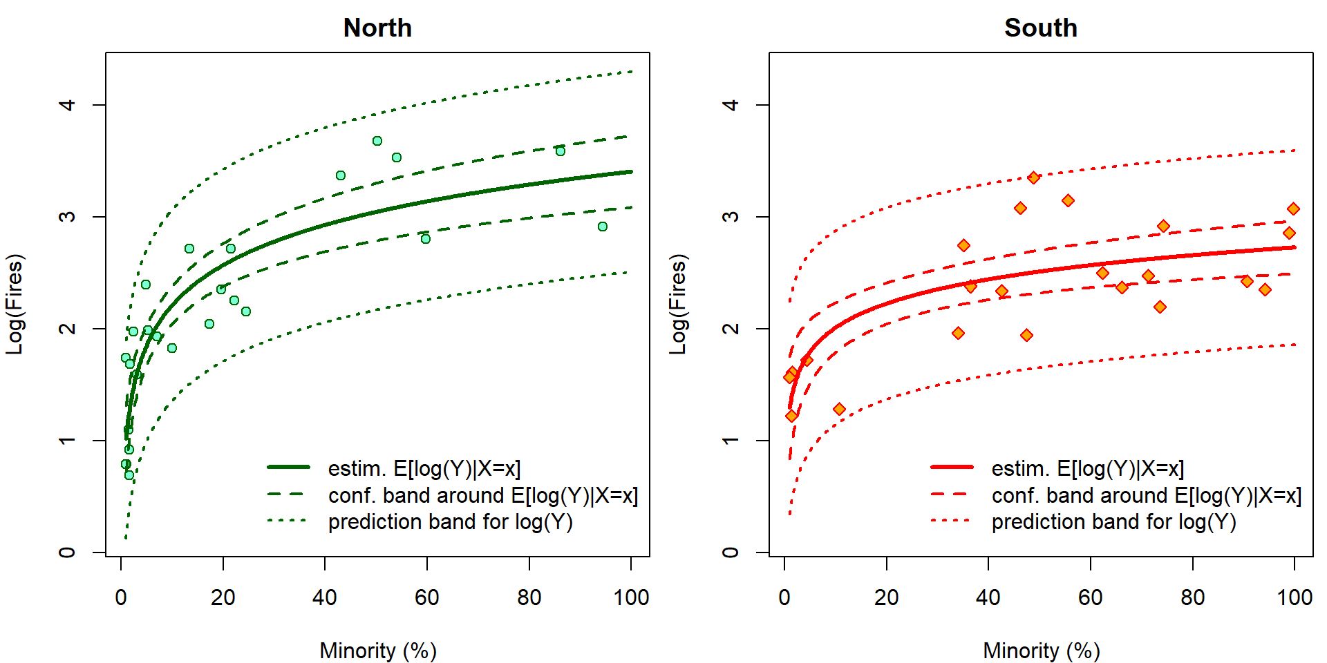
The confidence intervals \[ \mathsf{P} \left( (LCI, UCI)\ni \mathbf{x}^\top \widetilde{\boldsymbol{\beta}} = \mathsf{E}\left[\log Y | \mathbf{X}= \mathbf{x} \right] \right) \] cannot be interpreted with respect to original scale by simple \(\exp\) transformation \[ \mathsf{P} \left( (\exp\{LCI\}, \exp\{UCI\})\ni \exp\{\mathbf{x}^\top \widetilde{\boldsymbol{\beta}}\} = \exp\left\{\mathsf{E}\left[\log Y | \mathbf{X}= \mathbf{x} \right]\right\} < \mathsf{E}\left[Y | \mathbf{X}= \mathbf{x} \right] \right). \] However, it still works for prediction intervals: \[ \mathsf{P} \left( \log Y_{new} \in (LPI, UPI) \right) = \mathsf{P} \left( Y_{new} \in (\exp\{LPI\}, \exp\{UPI\}) \right). \] Now we plot the same outputs but on original scales. Grey colors correspond to incorrect estimates for \(\exp {\mathsf{E} [\log Y | \mathbf{X} ]}\) that are simple \(\exp\) transformation of the estimates for \(\mathsf{E} [\log Y | \mathbf{X} ]\). Using \(\Delta\)-method and knowledge of log-normal distribution, \(\mathsf{E} \exp{ \varepsilon} = \exp \left\{\frac{\sigma^2}{2}\right\}\), we can calculate the true estimates for \(\mathsf{E} \left[ Y | \mathbf{X}\right]\) (colourful).

YLIM <- range(chicago[, "fire"], exp(pfit))
XLIM <- range(chicago[, "minor"])

# True point estimate and CI for E[Y|X] based on log-N distribution
sigma2 <- summary(m)$sigma^2
EYX_fit <- exp(cifit$fit[,"fit"] + sigma2/2)
CIEYX_lwr <- EYX_fit * (1 - qnorm(0.975) * cifit$se.fit)
CIEYX_upr <- EYX_fit * (1 + qnorm(0.975) * cifit$se.fit)

par(mfrow = c(1, 2), mar=c(4,4,2,0.5))
for (ss in levels(chicago[, "fside"])){
  plot(fire ~ minor, data = subset(chicago, fside == ss), main = ss,
       xlab = XLAB, ylab = "Fires", xlim = XLIM, ylim = YLIM,
       col = COLS[fside], bg = BGS[fside], pch = PCHS[fside])
  ind <- if (ss == "North") 1:lpred else (lpred + 1):(2 * lpred)
  lines(pminor, exp(cifit$fit[ind, "fit"]), col = "grey30", lwd = 3)
  lines(pminor, exp(cifit$fit[ind, "lwr"]), col = "grey40", lwd = 2, lty = 2)
  lines(pminor, exp(cifit$fit[ind, "upr"]), col = "grey40", lwd = 2, lty = 2)
  lines(pminor, EYX_fit[ind], col = COLS[ss], lwd = 3)
  lines(pminor, CIEYX_lwr[ind], col = COLS[ss], lwd = 2, lty = 2)
  lines(pminor, CIEYX_upr[ind], col = COLS[ss], lwd = 2, lty = 2)
  lines(pminor, exp(pfit[ind, "lwr"]), col = COLS[ss], lwd = 2, lty = 3)
  lines(pminor, exp(pfit[ind, "upr"]), col = COLS[ss], lwd = 2, lty = 3)
  
    legend("topleft", bty = "n",
           legend=c("estim. exp(E[log(Y)|X=x]) < E[Y|X=x]",
                    "conf. band around exp(E[log(Y)|X=x]) < E[Y|X=x]",
                    "estim. E[Y|X=x]",
                    "conf. band around E[Y|X=x]",
                    "prediction band for Y"),
           lwd=c(3,2,3,2,2), lty=c(1,2,1,2,3), 
           col=c("grey30","grey40",COLS[ss],COLS[ss],COLS[ss])) 
}

Model assumptions and graphical diagnostic tools

Jan Vávra

Exercise 9

Loading the data and libraries

1. Basic model diagnostics

Individual work

2. Fitting correct \(E[Y \mid \mathbf{X}]\)

Polynomials and splines

Individual work

3. Log transformation of the response

Exploration

Interpretation of a model with log-transformed response