Simple (ordinary) linear regression model for a continuous variable

Download this R markdown as: R, Rmd.

Outline of the lab session:

Simple (ordinary) linear regression model for a continuous variable $Y \in \mathbb{R}$

the explanatory variable $X \in \mathbb{R}$ is continuous,
the explanatory variable $X \in \mathbb{R}$ is binary,
transformations of the explanatory variable.

Loading the data and libraries

Some necessary R packages (each package must be firstly installed in R – this can be achieved by running the command install.packages("package_name")). After the installation, the libraries are initialized by

library(MASS)
library(ISLR2)

The installation (command install.packages()) should be performed just once. However, the initialization of the library – the command library() – must be used every time when starting a new R session.

1. Simple (ordinary) linear regression

The ISLR2 library contains the Boston data set, which records medv (median house value) for $506$ census tracts in Boston. We will seek to predict medv using some of the $12$ given predictors such as rm (average number of rooms per house), age (average age of houses), or lstat (percent of households with low socioeconomic status).

head(Boston)

##      crim zn indus chas   nox    rm  age    dis rad tax ptratio lstat medv
## 1 0.00632 18  2.31    0 0.538 6.575 65.2 4.0900   1 296    15.3  4.98 24.0
## 2 0.02731  0  7.07    0 0.469 6.421 78.9 4.9671   2 242    17.8  9.14 21.6
## 3 0.02729  0  7.07    0 0.469 7.185 61.1 4.9671   2 242    17.8  4.03 34.7
## 4 0.03237  0  2.18    0 0.458 6.998 45.8 6.0622   3 222    18.7  2.94 33.4
## 5 0.06905  0  2.18    0 0.458 7.147 54.2 6.0622   3 222    18.7  5.33 36.2
## 6 0.02985  0  2.18    0 0.458 6.430 58.7 6.0622   3 222    18.7  5.21 28.7

To find out more about the data set, we can type ?Boston.

We will start with some simple explanatory analysis. For all three explanatory variables we draw a simple scatterplot.

par(mfrow = c(1,3), mar = c(4,4,0.5,0.5))
plot(medv ~ rm, data = Boston, pch = 22, bg = "gray", 
     ylab = "Median value [in 1000$]", xlab = "Average number of rooms")
plot(medv ~ age, data = Boston, pch = 22, bg = "gray", 
     ylab = "", xlab = "Proportion of owner-occupied units built prior to 1940")
plot(medv ~ lstat, data = Boston, pch = 22, bg = "gray", 
     ylab = "", xlab = "Lower status of the population [%].")

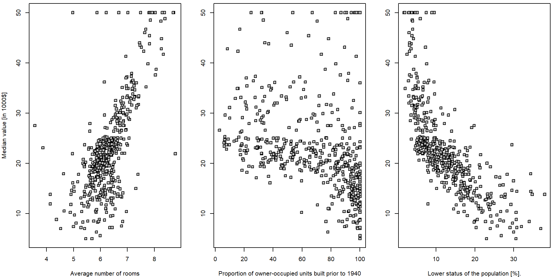
It seems that there is a positive (progressive) relationship between the median house value (dependent variable medv) and the average number of room in the house (independent variable rm) and a negative relationship (regression) in terms of the relationship between the median house value and the population status (explanatory variable lstat). For the proportion of the owner-occupied units build prior to 1940 (variable age), it is not that much obvious what relationship to expect… In all three situations we will go for a simple linear (ordinary) regression model in terms of

$Y_i = a + b X_i + \varepsilon_i \qquad i = 1, \dots, 506.$

Individual work

For all four covariates of interest (one dependent variable and three independent variables) perform a simple exploratory analysis in terms of some estimated characteristics (e.g., the estimate for mean, median, variance, standard error).
Use some graphical tools to visualize the structure in the given data – the four covariates of interest (e.g. some simple boxplots).
Perform a more detailed exploratory analysis in terms of splitting the data into some reasonable subgroups and estimated the corresponding characteristics in each subgroup separately (for instance, you can consider two subgroups by distinguishing the proportion age below 50% and above 50%).

vars <- c("medv", "rm", "age", "lstat")
summary(Boston[,vars])

##       medv             rm             age             lstat      
##  Min.   : 5.00   Min.   :3.561   Min.   :  2.90   Min.   : 1.73  
##  1st Qu.:17.02   1st Qu.:5.886   1st Qu.: 45.02   1st Qu.: 6.95  
##  Median :21.20   Median :6.208   Median : 77.50   Median :11.36  
##  Mean   :22.53   Mean   :6.285   Mean   : 68.57   Mean   :12.65  
##  3rd Qu.:25.00   3rd Qu.:6.623   3rd Qu.: 94.08   3rd Qu.:16.95  
##  Max.   :50.00   Max.   :8.780   Max.   :100.00   Max.   :37.97

apply(Boston[,vars], 2, sd)

##       medv         rm        age      lstat 
##  9.1971041  0.7026171 28.1488614  7.1410615

cor(Boston[,vars])

##             medv         rm        age      lstat
## medv   1.0000000  0.6953599 -0.3769546 -0.7376627
## rm     0.6953599  1.0000000 -0.2402649 -0.6138083
## age   -0.3769546 -0.2402649  1.0000000  0.6023385
## lstat -0.7376627 -0.6138083  0.6023385  1.0000000

for(x in vars[2:4]){
  Boston[,paste0("f",x)] <- cut(Boston[,x], breaks = quantile(Boston[,x], seq(0,1, length.out = 5)))
}

fxs <- paste0("f",vars[2:4])
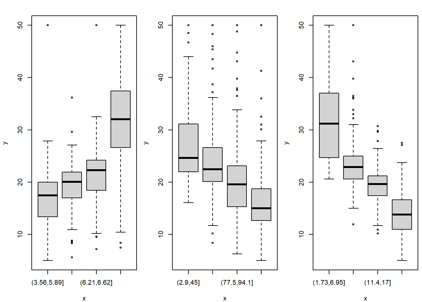
summary(Boston[,fxs])

##           frm               fage             flstat   
##  (3.56,5.89]:126   (2.9,45]   :126   (1.73,6.95]:126  
##  (5.89,6.21]:126   (45,77.5]  :126   (6.95,11.4]:126  
##  (6.21,6.62]:126   (77.5,94.1]:126   (11.4,17]  :126  
##  (6.62,8.78]:127   (94.1,100] :127   (17,38]    :127  
##  NA's       :  1   NA's       :  1   NA's       :  1

par(mfrow = c(1,3), mar = c(4,4,2,0.5))
for(x in fxs){
  plot(x = Boston[,x], y = Boston$medv)
}

In order to get some insight into the relationship $Y = f(X) + \varepsilon$ (and to judge the appropriateness of the linear line to be used as a surrogate for $f(\cdot)$ ) we can take a look at some (non-parametric) data smoothing – function lowess() in R:

par(mfrow = c(1,3), mar = c(4,4,0.5,0.5))
plot(medv ~ rm, data = Boston, pch = 22, bg = "gray", 
     ylab = "Median value [in 1000$]", xlab = "Average number of rooms")
lines(lowess(Boston$medv ~ Boston$rm, f = 2/3), col = "red", lwd = 2)
plot(medv ~ age, data = Boston, pch = 22, bg = "gray", 
     ylab = "", xlab = "Proportion of owner-occupied units built prior to 1940")
lines(lowess(Boston$medv ~ Boston$age, f = 2/3), col = "red", lwd = 2)
plot(medv ~ lstat, data = Boston, pch = 22, bg = "gray", 
     ylab = "", xlab = "Lower status of the population [%].")
lines(lowess(Boston$medv ~ Boston$lstat, f = 2/3), col = "red", lwd = 2)

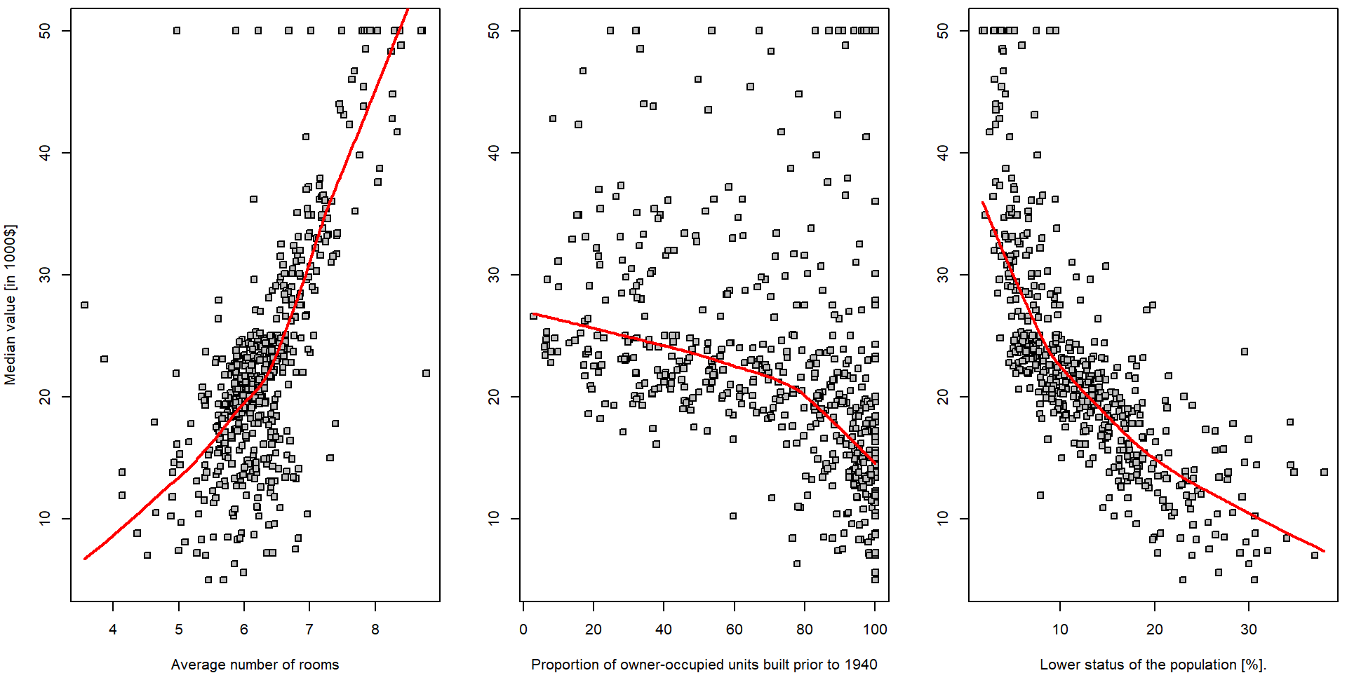
Note, that there is hardly any reasonable analytical expression for the red curves above (the specific form of the function $f(\cdot)$ ). Also note the parameter f = 2/3 in the function lowess(). Run the same R code with different options for the value of this parameter to see differences.

Explanatory variable `lstat`

We will now fit a simple linear regression line through the data using the R function lm(). In the implementation used below, the analytical form of the function $f(\cdot)$ being used to “smooth” the data is $f(x) = a + bx$ for some intercept parameter $a \in \mathbb{R}$ and the slope parameter $b \in \mathbb{R}$ . The following R code fits a simple linear regression line, with medv as the response (depedent variable) and lstat as the predictor (explanatory/indepenent variable/covariate). The basic syntax is lm(y ~ x, data), where y is the response, x is the predictor, and data is the data set in which these two variables are kept.

lm.fit <- lm(medv ~ lstat, data = Boston)

If we type lm.fit, some basic information about the model is output. For more detailed information, we use summary(lm.fit). This gives us $p$ -values and standard errors for the coefficients, as well as the $R^2$ statistic and $F$ -statistic for the model.

lm.fit

## 
## Call:
## lm(formula = medv ~ lstat, data = Boston)
## 
## Coefficients:
## (Intercept)        lstat  
##       34.55        -0.95

This fits a straight line through the data (the line intersects the $y$ axis at the point $34.55$ and the value of the slope parameter – which equals $-0.95$ – means that for each unit increase on the $x$ axis the line drops by $0.95$ units with respect to the $y$ axis).

par(mfrow = c(1,1), mar = c(4,4,0.5,0.5))
plot(medv ~ lstat, data = Boston, pch = 22, bg = "gray", 
     ylab = "Median value [in 1000$]", xlab = "Lower status of the population [%].")
lines(lowess(Boston$medv ~ Boston$lstat, f = 2/3), col = "red", lwd = 2)
abline(lm.fit, col = "blue", lwd = 2)

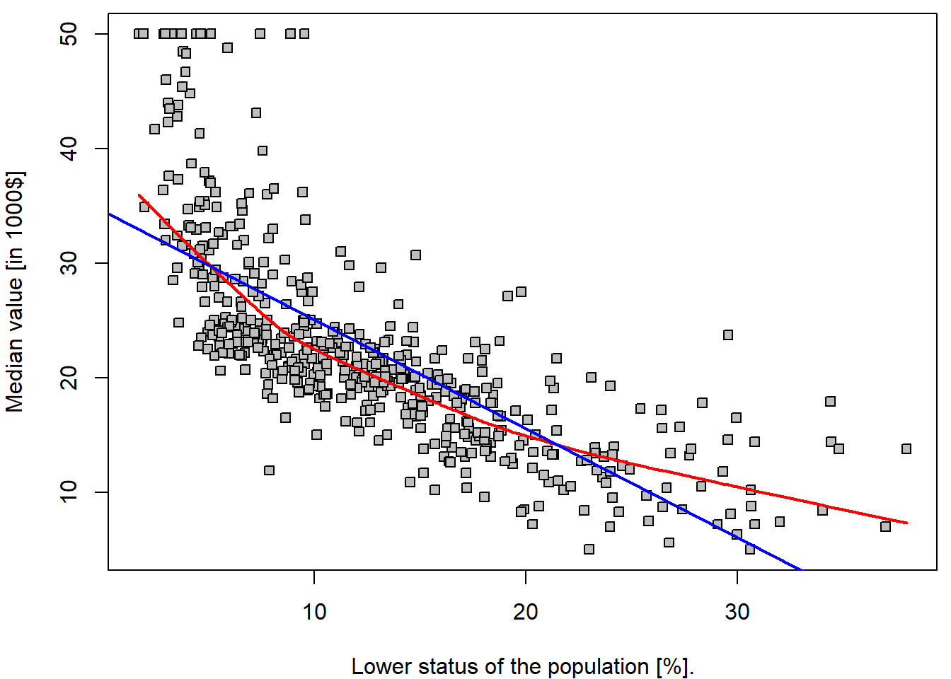
It is important to realize that the estimated parameters $34.55$ and $-0.95$ are given realization of two random variables – $\widehat{a}$ and $\widehat{b}$ (i.e., for another dataset, or another subset of the observations we would obtained different values of the estimated parameters). Thus, we are speaking about random quantities here and, therefore, it is reasonable to inspect some of their statistical properties (such as the corresponding mean parameters, variance of the estimates, or even their full distribution…).

Some of the statistical properties (i.e., the empirical estimates for the standard errors of the estimates) can be obtained by the following command:

(sum.lm.fit <- summary(lm.fit))

## 
## Call:
## lm(formula = medv ~ lstat, data = Boston)
## 
## Residuals:
##     Min      1Q  Median      3Q     Max 
## -15.168  -3.990  -1.318   2.034  24.500 
## 
## Coefficients:
##             Estimate Std. Error t value Pr(>|t|)    
## (Intercept) 34.55384    0.56263   61.41   <2e-16 ***
## lstat       -0.95005    0.03873  -24.53   <2e-16 ***
## ---
## Signif. codes:  0 '***' 0.001 '**' 0.01 '*' 0.05 '.' 0.1 ' ' 1
## 
## Residual standard error: 6.216 on 504 degrees of freedom
## Multiple R-squared:  0.5441, Adjusted R-squared:  0.5432 
## F-statistic: 601.6 on 1 and 504 DF,  p-value: < 2.2e-16

We can use the names() function in order to find out what other pieces of information are stored in lm.fit. Although we can extract these quantities by name—e.g. lm.fit$coefficients—it is safer to use the extractor functions like coef() to access them.

names(lm.fit)

##  [1] "coefficients"  "residuals"     "effects"       "rank"          "fitted.values" "assign"       
##  [7] "qr"            "df.residual"   "xlevels"       "call"          "terms"         "model"

coef(lm.fit)

## (Intercept)       lstat 
##  34.5538409  -0.9500494

It is important to realize, that the estimates $\widehat{a}$ and $\widehat{b}$ are random variables. They have the corresponding variances $\mathsf{var} (\widehat{a})$ and $\mathsf{var} (\widehat{b})$ but the values that we see in the table above are just the estimates of this theoretical quantities – thus, mathematically correctly, we should use the notation $\widehat{\mathsf{var}(\widehat{a})} \approx 0.5626^2 \qquad\text{and}\qquad \widehat{\mathsf{var}(\widehat{b})} \approx 0.03873^2$ The values in the table (second column) are the estimates for the true standard errors of $\widehat{a}$ and $\widehat{b}$ (because we do not now the true variance, or standard error respectively, of the error terms $\varepsilon_i$ in the underlying model $Y_i = a + b X_i + \varepsilon_i$ , where we only assume that $\varepsilon_i \sim (0, \sigma^2)$ ).

The unknown variance $\sigma^2 > 0$ is also estimated in the output above – see the value for the Residual standard error. Thus, we have $\widehat{\sigma^2} = 6.216^2$ .

### model residuals -- estimates for random errors and their estimated variance/standard error
var(lm.fit$residuals)

## [1] 38.55917

sqrt(var(lm.fit$residuals))   # not exactly as in summary, var divides by (n-1) not (n-rank)

## [1] 6.209603

The intercept parameter $a \in \mathbb{R}$ and the slope parameter $b \in \mathbb{R}$ are unknown but fixed parameters and we have the corresponding (point) estimates for both – random quantities $\widehat{a}$ and $\widehat{b}$ . Thus, it is also reasonable to ask for an interval estimates instead – the confidence intervals for $a$ and $b$ .
This can be obtained by the command confint().

confint(lm.fit)

##                 2.5 %     97.5 %
## (Intercept) 33.448457 35.6592247
## lstat       -1.026148 -0.8739505

The estimated parameters $\widehat{a}$ and $\widehat{b}$ can be used to estimate some characteristic of the distribution of the dependent variable $Y$ (i.e., medv) given the value of the independent variable “ $X = x$ ” (i.e., lstat). In other words, the estimated parameters can be used to estimate the conditional expectation of the conditional distribution of $Y$ given “ $X = x$ ”, respectively $\widehat{\mu_x} = \widehat{E[Y | X = x]} = \widehat{a} + \widehat{b}x.$

However, sometimes it can be also useful to “predict” the value of $Y$ for a specific value of $X$ . As far as $Y$ is random (even conditionally on $X = x$ ) we need to give some characteristic of the whole conditional distribution – and this characteristic is said to be a prediction for $Y$ . It is common to use the conditional expectation for this purpose.

In the R program, we can use the predict() function, which also produce the confidence intervals and prediction intervals for the prediction of medv for a given value of lstat.

(pred.conf <- predict(lm.fit, data.frame(lstat = (c(5, 10, 15))), interval = "confidence"))

##        fit      lwr      upr
## 1 29.80359 29.00741 30.59978
## 2 25.05335 24.47413 25.63256
## 3 20.30310 19.73159 20.87461

(pred.pred <- predict(lm.fit, data.frame(lstat = (c(5, 10, 15))), interval = "prediction"))

##        fit       lwr      upr
## 1 29.80359 17.565675 42.04151
## 2 25.05335 12.827626 37.27907
## 3 20.30310  8.077742 32.52846

For instance, the 95,% confidence interval associated with a lstat value of 10 is $(24.47, 25.63)$ , and the 95,% prediction interval is $(12.83, 37.28)$ . As expected, the confidence and prediction intervals are centered around the same point (a predicted value of $25.05$ for medv when lstat equals 10), but the latter are substantially wider. Can you explain why?

Individual work

Add confidence and prediction intervals to the fitted line.

grid <- 0:100
pred_conf <- predict(lm.fit, newdata = data.frame(lstat = grid), interval = "confidence")
pred_pred <- predict(lm.fit, newdata = data.frame(lstat = grid), interval = "predict")

par(mfrow = c(1,1), mar = c(4,4,0.5,0.5))
plot(medv ~ lstat, data = Boston, pch = 22, bg = "gray", 
     ylab = "Median value [in 1000$]", xlab = "Lower status of the population [%].")
lines(lowess(Boston$medv ~ Boston$lstat, f = 2/3), col = "red", lwd = 2)
abline(lm.fit, col = "blue", lwd = 2)
lines(x = grid, y = pred_conf[,"lwr"], col = "darkviolet", lty = 2, lwd = 2)
lines(x = grid, y = pred_conf[,"upr"], col = "darkviolet", lty = 2, lwd = 2)
lines(x = grid, y = pred_pred[,"lwr"], col = "chocolate", lty = 3, lwd = 2)
lines(x = grid, y = pred_pred[,"upr"], col = "chocolate", lty = 3, lwd = 2)

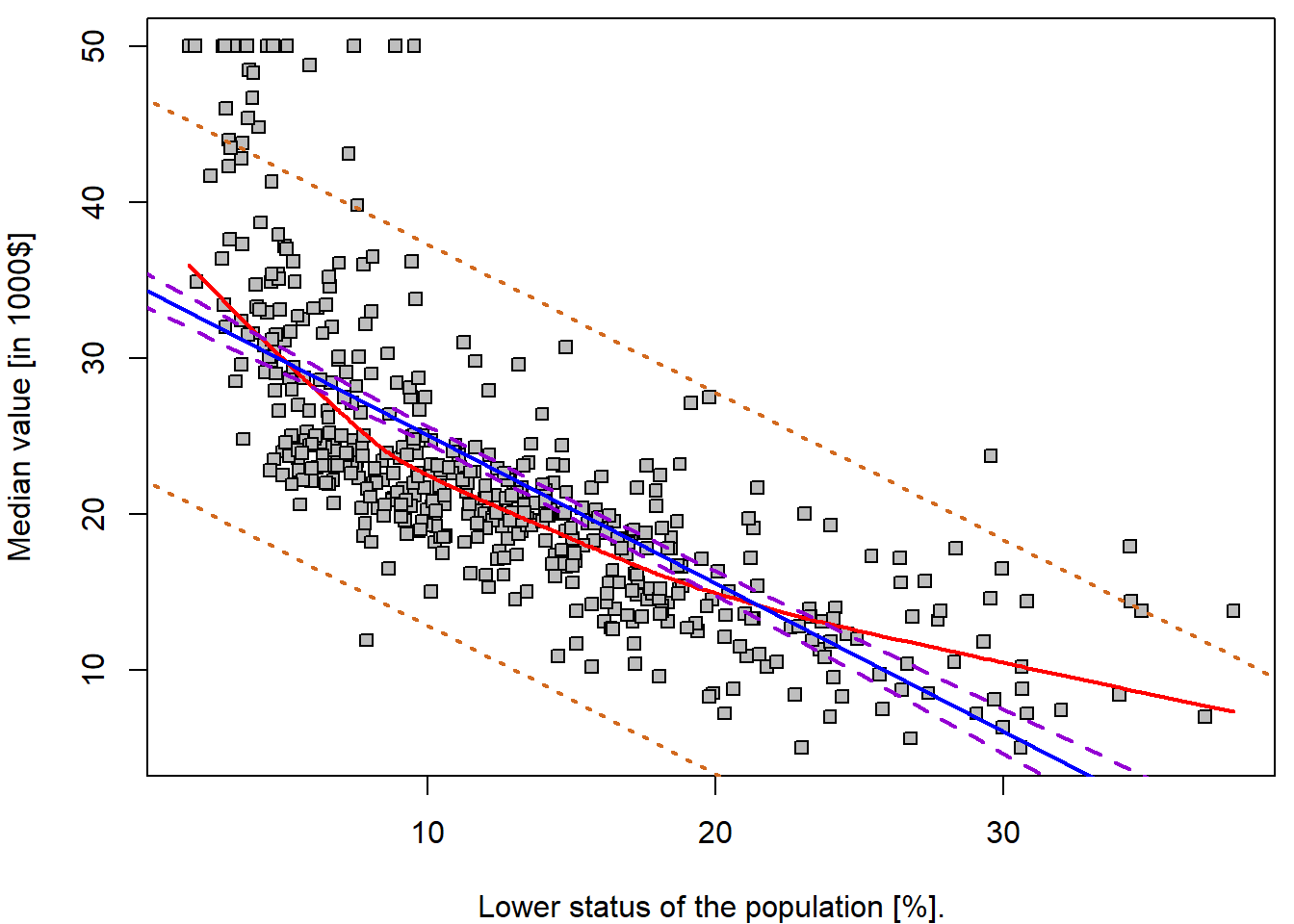
Some “goodness-of-fit” diagnostics

Next we examine some diagnostic plots – but we will discuss different diagnostics tools later.

Four diagnostic plots are automatically produced by applying the plot() function directly to the output from lm(). In general, this command will produce one plot at a time, and hitting Enter will generate the next plot. However, it is often convenient to view all four plots together. We can achieve this by using the par() and mfrow() functions, which tell R to split the display screen into separate panels so that multiple plots can be viewed simultaneously. For example, par(mfrow = c(2, 2)) divides the plotting region into a $2 \times 2$ grid of panels:

par(mfrow = c(2, 2), mar = c(4,4,2,0.5))
plot(lm.fit)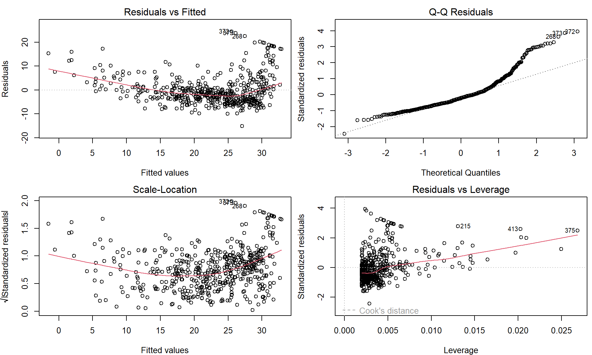

These plots can be used to judge the quality of the model that was used – in our particular case we used a simple linear regression line of the form $Y = a + bX + \varepsilon$ .

Individual work

Repeat the previous R code and fit simple linear regression models also for the remaining explanatory variable mentioned at the beginning – age and rm.
Compare the quality of all three models – visually by looking at the scatterplot and the fitted line and, also, by looking at four diagnostic plots as shown above.
Which of the three models is the one that you consider the most reliable? Which one do you consider mostly unreliable?
Is there any relationship/expectation with respect to the estimated covariances and correlations below?

cov(Boston$medv, Boston$rm)

## [1] 4.493446

cov(Boston$medv, Boston$age)

## [1] -97.58902

cov(Boston$medv, Boston$lstat)

## [1] -48.44754

cor(Boston$medv, Boston$rm)

## [1] 0.6953599

cor(Boston$medv, Boston$age)

## [1] -0.3769546

cor(Boston$medv, Boston$lstat)

## [1] -0.7376627

2. Binary explanatory variable $X$

Until now, the explanatory variable $X$ was treated as a continuous variable. However, this variable can be also used as a binary information (and also as a categorical variable, but this will be discussed later).

We already mentioned a situation where the proportion of the owner-occupied houses is below 50% and above. Thus, we will create another variable in the original data that will reflect this information.

Boston$fage <- (Boston$age > 50)
table(Boston$fage)

## 
## FALSE  TRUE 
##   147   359

We can look at both subpopulations by the means of two boxplots for instance:

par(mfrow = c(1,1), mar = c(4,4,0.5,0.5))
boxplot(medv ~ fage, data = Boston, col = "lightblue", 
        xlab = "Proportion of owner-occupied houses prior to 1940 is above 50%", ylab = "Median house value")

The figure above somehow corresponds with the scatterplot of medv against age where we observed that higher proportion (i.e., higher values of the age variable) are associated with rather lower median house values (dependent variable $Y \equiv$ medv). In the boxplot above, we can also see that higher proportions of the owner-occupied houses prior to 1940 (the sub-population where the proportion is above $50\%$ ) are associated with rather lower median house values.

What will happen when this information (explanatory variable fage which only takes two values – one for true and zero otherwise) will be used in a simple linear regression model?

lm.fit2 <- lm(medv ~ fage, data = Boston)
lm.fit2

## 
## Call:
## lm(formula = medv ~ fage, data = Boston)
## 
## Coefficients:
## (Intercept)     fageTRUE  
##      26.693       -5.864

And the correponding statistical summary of the model:

summary(lm.fit2)

## 
## Call:
## lm(formula = medv ~ fage, data = Boston)
## 
## Residuals:
##     Min      1Q  Median      3Q     Max 
## -15.829  -5.720  -1.729   2.898  29.171 
## 
## Coefficients:
##             Estimate Std. Error t value Pr(>|t|)    
## (Intercept)  26.6932     0.7267  36.730  < 2e-16 ***
## fageTRUE     -5.8639     0.8628  -6.796 3.04e-11 ***
## ---
## Signif. codes:  0 '***' 0.001 '**' 0.01 '*' 0.05 '.' 0.1 ' ' 1
## 
## Residual standard error: 8.811 on 504 degrees of freedom
## Multiple R-squared:  0.08396,    Adjusted R-squared:  0.08214 
## F-statistic: 46.19 on 1 and 504 DF,  p-value: 3.038e-11

Can you see some analogy with the following (partial) exploratory characteristic (respectively their sample estimates)?

mean(Boston$medv[Boston$fage == F])

## [1] 26.6932

mean(Boston$medv[Boston$fage == T])

## [1] 20.82925

mean(Boston$medv[Boston$fage == T]) - mean(Boston$medv[Boston$fage == F])

## [1] -5.863949

The estimated model in this case takes a form $Y = a + bX + \varepsilon$ where $x$ can only take two specific values – it is either equal to zero and, thus, the model becomes $f(x) = a$ or the value of $x$ is equal to 1 and the model becomes $f(x) = a + b$ . Note, that any other parametrization of the explanatory variable $X$ (for instance, $x = -1$ for the subpopulation with the proportion below 50% and $x = 1$ for the subpopulation with the proportion above 50%) gives mathematically equivalent model.

### different parametrization of two subpopulations (using +/- 1 instead of 0/1)
Boston$fage2 <- (2 * as.numeric(Boston$fage) - 1)
head(Boston)

##      crim zn indus chas   nox    rm  age    dis rad tax ptratio lstat medv         frm  fage      flstat
## 1 0.00632 18  2.31    0 0.538 6.575 65.2 4.0900   1 296    15.3  4.98 24.0 (6.21,6.62]  TRUE (1.73,6.95]
## 2 0.02731  0  7.07    0 0.469 6.421 78.9 4.9671   2 242    17.8  9.14 21.6 (6.21,6.62]  TRUE (6.95,11.4]
## 3 0.02729  0  7.07    0 0.469 7.185 61.1 4.9671   2 242    17.8  4.03 34.7 (6.62,8.78]  TRUE (1.73,6.95]
## 4 0.03237  0  2.18    0 0.458 6.998 45.8 6.0622   3 222    18.7  2.94 33.4 (6.62,8.78] FALSE (1.73,6.95]
## 5 0.06905  0  2.18    0 0.458 7.147 54.2 6.0622   3 222    18.7  5.33 36.2 (6.62,8.78]  TRUE (1.73,6.95]
## 6 0.02985  0  2.18    0 0.458 6.430 58.7 6.0622   3 222    18.7  5.21 28.7 (6.21,6.62]  TRUE (1.73,6.95]
##   fage2
## 1     1
## 2     1
## 3     1
## 4    -1
## 5     1
## 6     1

lm.fit3 <- lm(medv ~ fage2, data = Boston)
lm.fit3

## 
## Call:
## lm(formula = medv ~ fage2, data = Boston)
## 
## Coefficients:
## (Intercept)        fage2  
##      23.761       -2.932

Individual work

Usually, with different parametrization we obtain different interpretation options and statistical characteristics for different quantities when calling the function summary().

What is the interpretation of the estimates $\widehat{a}$ and $\widehat{b}$ in this case?
Recall, that the model $f(x) = a + bx$ for $x = \pm 1$ takes now the form $f(x) = a - b$ if the proportion is below $50\%$ and the model becomes $f(x) = a + b$ if the proportion is above $50\%$ .
Can you reconstruct both estimates for subpopulations means using the model above?
Try to think of some other parametrization of the independent variable $X$ (the information whether the proportion is above or below $50\%$ ).
In the model above we have the estimate for the intercept parameter $\widehat{a} = 23.76$ . Can you guess what does it stands for? What theoretical characteristic does it estimate?

(mean(Boston$medv[Boston$fage2 == -1]) + mean(Boston$medv[Boston$fage2 == 1]))/2

## [1] 23.76122

Recall, that two subpopulations are not equal with respect to their size. What would be estimated by the intercept parameter estimate $\widehat{a}$ if both subpopulations would be equal with respect to the size (i.e., balanced data)?
Compare summary() outputs for the two models. Which quantities are the same for both parametrizations?
How would you fit a model where coefficients correspond to individual groups (no intercept)?

3. Transformations of the predictor variable $X$

We already mentioned some transformation (parametrizations) of the independent/exploratory variable $X$ in a situation where $X$ stands for a binary information (yes/no, true/false, $\pm 1$ , $0/1$ , etc.). However, different transformations can be also used for the independent covariate $X$ if it stands for a continuous variable.

Consider the first model

lm.fit

## 
## Call:
## lm(formula = medv ~ lstat, data = Boston)
## 
## Coefficients:
## (Intercept)        lstat  
##       34.55        -0.95

and the model

lm(medv ~ I(lstat/100), data = Boston)

## 
## Call:
## lm(formula = medv ~ I(lstat/100), data = Boston)
## 
## Coefficients:
##  (Intercept)  I(lstat/100)  
##        34.55        -95.00

What type of transformation is used in this example and what is the underlying interpretation of this different parametrization of $X$ ? Such and similar parametrization are typically used to improve the interpretation of the final model. For instance, using the first model lm.fit the interpretation of the estimated intercept parametr $\widehat{a}$ can be given as follows: “The estimated expected value for the median house value is 34.5 thousand dollars if the lower population status is at the zero level.” But this may not be realistic when looking at the data – indeed, the minimum observed value for lstat is $1.73$ . Thus, it can be more suitable to use a different interpretation of the intercept parameter. Consider the following model and the summary statistics for lstat:

lm(medv ~ I(lstat - 11.36), data = Boston)

## 
## Call:
## lm(formula = medv ~ I(lstat - 11.36), data = Boston)
## 
## Coefficients:
##      (Intercept)  I(lstat - 11.36)  
##            23.76             -0.95

summary(Boston$lstat)

##    Min. 1st Qu.  Median    Mean 3rd Qu.    Max. 
##    1.73    6.95   11.36   12.65   16.95   37.97

What is the interpretation of the intercept parameter estimate in this case? Can you obtain the value of the estimate using the original model?

The transformations of the independent covariates can be, however, also used to improve the model fit. For instance, consider the following model

Boston$lstat_transformed <- sqrt(Boston$lstat)
lm.fit4 <- lm(medv ~ lstat_transformed, data = Boston)

Both model can be compared visually:

par(mfrow = c(1,3), mar = c(4,4,2,0.5))
plot(medv ~ lstat, data = Boston, pch = 22, bg = "gray", 
     ylab = "Median value [in 1000$]", xlab = "Lower status of the population [%].",
     main = "Original scale X - linear trend")
abline(lm.fit, col = "blue", lwd = 2)

plot(medv ~ lstat_transformed, data = Boston, pch = 22, bg = "gray", 
     ylab = "", xlab = "Lower status of the population squared [sqrt(%)].",
     main = "Square root of X")
abline(lm.fit4, col = "blue", lwd = 2)

plot(medv ~ lstat, data = Boston, pch = 22, bg = "gray", 
     ylab = "", xlab = "Lower status of the population [%].",
     main = "Sqrt X fit on original scale")
xGrid <- seq(0,40, length = 1000)
yValues <- lm.fit4$coeff[1] + lm.fit4$coeff[2] * sqrt(xGrid)
lines(yValues  ~ xGrid, col = "blue", lwd = 2)

Note, that the first plot is the scatterplot for the relationship medv $\sim$ lstat – which is the original model which fits the straight line through the data. The middle plot is the scatterplot for the relationship medv $\sim ($ lstat $)^{1/2}$ and the corresponding model (lm.fit4) again fits the straight line through the data (with coordinates $(Y_i, \sqrt{X_i})$ ). Finally, the third plot shows the original scatterplot (the data with the coordinates $(Y_i, X_i)$ ) but the model lm.fit4 does not fit a straight line through such data. The interpretation is simple with respect to the transformed data $(Y_i, \sqrt{X_i})$ but it is not that much straightforward with respect to the original data $(Y_i, X_i)$ .

Nevertheless, it seems that the model lm.fit4 fits the data more closely that the model lm.fit.

Individual work

Think of some alternative transformation of the original data in order to improve the overall fit of the model.
Do not care for the interpretation issues for now, only focus on some reasonable approximation that will help to improve the quality of the fit.
Try to obtain some quantitative characteristic for the quality of the fits – for instance, the residual sum of squares.

Simple (ordinary) linear regression model for a continuous variable

Jan Vávra

Exercise 3

Outline of the lab session:

Loading the data and libraries

1. Simple (ordinary) linear regression

Individual work

Explanatory variable `lstat`

Individual work

Some “goodness-of-fit” diagnostics

Individual work

2. Binary explanatory variable $X$

Individual work

3. Transformations of the predictor variable $X$

Individual work

Simple (ordinary) linear regression model for a continuous variable

Jan Vávra

Exercise 3

Outline of the lab session:

Loading the data and libraries

1. Simple (ordinary) linear regression

Individual work

Explanatory variable lstat

Individual work

Some “goodness-of-fit” diagnostics

Individual work

2. Binary explanatory variable XX

Individual work

3. Transformations of the predictor variable XX

Individual work

Explanatory variable `lstat`

2. Binary explanatory variable $X$

3. Transformations of the predictor variable $X$