Bayesian Methods - Ex3d - Joint Model (again)
Jan Vávra
The goal of this exercise is to demonstrate the use of packages
JM and JMbayes for fitting joint models
pursued by JAGS in Exercise
3c. No report is required, just admire the simplicity of the
solution (compared to JAGS).
Data and model description
We once again analyze the aids data from
library(JM), see help(aids) for more
details.
set.seed(123456789)
library(JM)
head(aids[,c("patient", "Time", "death", "CD4", "obstime", "drug", "start", "stop", "event")], 15)
## patient Time death CD4 obstime drug start stop event
## 1 1 16.97 0 10.677078 0 ddC 0 6.00 0
## 2 1 16.97 0 8.426150 6 ddC 6 12.00 0
## 3 1 16.97 0 9.433981 12 ddC 12 16.97 0
## 4 2 19.00 0 6.324555 0 ddI 0 6.00 0
## 5 2 19.00 0 8.124038 6 ddI 6 12.00 0
## 6 2 19.00 0 4.582576 12 ddI 12 18.00 0
## 7 2 19.00 0 5.000000 18 ddI 18 19.00 0
## 8 3 18.53 1 3.464102 0 ddI 0 2.00 0
## 9 3 18.53 1 3.605551 2 ddI 2 6.00 0
## 10 3 18.53 1 6.164414 6 ddI 6 18.53 1
## 11 4 12.70 0 3.872983 0 ddC 0 2.00 0
## 12 4 12.70 0 4.582576 2 ddC 2 6.00 0
## 13 4 12.70 0 2.645751 6 ddC 6 12.00 0
## 14 4 12.70 0 1.732051 12 ddC 12 12.70 0
## 15 5 15.13 0 7.280110 0 ddI 0 2.00 0Let us recall the model we were able to fit with JAGS in Exercise
3c. For CD4 variable, we assume LME model with random
intercept and slope:
- \(Y_{ij} = m_i(t_{ij}) + \varepsilon_{ij}
= B_{1i} + B_{2i} t_{ij} + \varepsilon_{ij}\), is the
CD4cell count of patient \(i\) at visit \(j\), - \(\varepsilon_{ij} \sim \mathsf{N}(0, \tau^{-1})\) is the iid model error,
- \(t_{ij}\) is the time of the observation of patient \(i\) at visit \(j\),
- \(D_i\) is the indicator of
druglevelddI, - \(B_{1i}\) and \(B_{2i}\) are the random intercept and slope for patient \(i\),
- \(\mathbf{B}_i = (B_{1i}, B_{2i})^\top \sim \mathsf{N}_2 \left(\begin{pmatrix} \beta_1 \\ \beta_2 + \beta_3 D_i \end{pmatrix}, \Sigma\right)\), where \(\Sigma\) is general positive-definite matrix.
According to this model, the expected CD4 cell count
\(m_i(t)\) evolves linearly with time
for each patient differently \(m_i(t) = B_{1i}
+ B_{2i} t\). This will monotonously project into the survival
probability of each patient.
Many patients leave the study prior their death, which leads to
right-censored data. The observed data are event times \(E_i = \min\{T_i, C_i\}\) and \(\delta_i = \mathbf{1} (T_i \leq C_i)\)
where \(C_i\) is assumed to be time of
censoring, independent of \(T_i\).
The distribution of time to death \(T_i\) for patient \(i\) is modelled through the hazard
function: \[\begin{align*}
h_i(t) &= h_0(t) \, \exp\left\{ \gamma_1 D_i + \gamma_2 m_i(t)
\right\} \\
&= h_0(t) \, \exp\left\{ \gamma_1 D_i + \gamma_2 B_{1i} + t \cdot
\gamma_2 B_{2i} \right\},
\end{align*}\] where we were able to implement only constant
\(h_0(t) = \xi\) or piecewise constant
baseline hazard function \(h_0(t) =
\prod\limits_{k=1}^{K} \xi_k^{\mathbf{1}(t_k < t \leq
t_{k+1})}\). The constant baseline hazard yields Gompertz
distribution with monotonous hazard function in time. The piecewise
constant baseline can adjust the monotonous exponential trend, but
cannot fully reverse the monotonicity for an interval.
According to smoothed derivative of Breslow estimator of
cumulative hazard function from classical semi-parametric Cox
proportional hazards model, the shape should resemble the following
shape:
 Such a shape calls for an even more flexible baseline hazard
parametrizations such as B-splines on log-scale. However, we will no
longer be able to find the closed formula for cumulative hazard \(H_i(t)\).
Such a shape calls for an even more flexible baseline hazard
parametrizations such as B-splines on log-scale. However, we will no
longer be able to find the closed formula for cumulative hazard \(H_i(t)\).
The likelihood function for observed data (in the general notation defined below) is of the following form: \[ p(\mathbb{Y}, \mathbf{E}, \boldsymbol{\delta} \,|\, \boldsymbol{\beta}, \sigma^2, \mathbb{D}, \boldsymbol{\gamma}, \alpha, \boldsymbol{\xi} \text{ or } \boldsymbol{\gamma}_{h_0}) = \\ = \prod\limits_{i=1}^n \int p(\mathbf{Y}_i | \mathbf{B}_i; \boldsymbol{\beta}, \sigma^2) \, \left[h_i(E_i | \mathbf{B}_i; \boldsymbol{\gamma}, \alpha, \boldsymbol{\xi} \text{ or } \boldsymbol{\gamma}_{h_0})\right]^{\delta_i} \, \exp\{-H_i(E_i | \mathbf{B}_i; \boldsymbol{\gamma}, \alpha, \boldsymbol{\xi} \text{ or } \boldsymbol{\gamma}_{h_0})\} \, p(\mathbf{B}_i | \mathbb{D}) \, \mathrm{d} \mathbf{B}_i \] where the individual contribution to log-likelihood is very complicated integral wrt random effects. For example, when B-spline basis is chosen for the log-baseline hazard, we obtain: \[ \ell(\mathbf{Y}_i, E_i, \delta_i \,|\, \boldsymbol{\beta}, \sigma^2, \mathbb{D}, \boldsymbol{\gamma}, \alpha, \boldsymbol{\gamma}_{h_0} ) = \\ = \log \left\langle\int \exp\left\{ \sum\limits_{j=1}^{n_i} \log p(Y_{ij} \mathbf{B}_i; \boldsymbol{\beta}, \sigma^2) + \delta_i \log h_i(E_i | \mathbf{B}_i; \boldsymbol{\gamma}, \alpha, \boldsymbol{\gamma}_{h_0}) - H_i(E_i | \mathbf{B}_i; \boldsymbol{\gamma}, \alpha, \boldsymbol{\gamma}_{h_0}) + \log p(\mathbf{B}_i | \mathbb{D}) \right\} \, \mathrm{d} \mathbf{B}_i \right\rangle = \\ = \log \left\langle \int \exp\left\{ -\frac{n_i}{2} \log (2\pi\sigma^2) - \frac{1}{2\sigma^2} \sum\limits_{j=1}^{n_i} \left[Y_{ij} - \mathbf{X}_i(t_{ij})^\top \boldsymbol{\beta} - \mathbf{Z}_i(t_{ij})^\top \mathbf{B}_i\right]^2 + \right. \right.\\ \left. + \delta_i \left[ \sum\limits_{q=1}^Q \gamma_{h_0,q} B_q^{\mathsf{spl}}(E_i;\mathbf{v}) + \mathbb{W}_i^\top \boldsymbol{\gamma} + \alpha \left( \mathbf{X}_i(E_i)^\top \boldsymbol{\beta} + \mathbf{Z}_i(E_i)^\top \mathbf{B}_i \right) \right] - \right. \\ \left. - \int\limits_0^{E_i} \exp \left[ \sum\limits_{q=1}^Q \gamma_{h_0,q} B_q^{\mathsf{spl}}(s;\mathbf{v}) + \mathbb{W}_i^\top \boldsymbol{\gamma} + \alpha \left( \mathbf{X}_i(s)^\top \boldsymbol{\beta} + \mathbf{Z}_i(s)^\top \mathbf{B}_i \right) \right] \, \mathrm{d} s - \right. \\ \left. \left. - \frac{1}{2} \log|\mathbb{D}| - \frac{1}{2} \mathbf{B}_i^{\top} \mathbb{D}^{-1} \mathbf{B}_i \right\} \, \mathrm{d} \mathbf{B}_i \right\rangle \] Hence, we need to resort to different R package(s) built for this exact purpose.
Joint model using libraries JM and JMbayes
JM in the name of these packages stands for
Joint Models. The two packages estimate the
joint models in two different approaches:
JMrelies on MLE, which is achieved by EM-algorithm and numerical approximation ((adaptive) Gaussian quadrature using Gauss-Hermite polynomials) of the integral wrt unobserved data (random effects and true survival times). Baseline hazard can be modelled by Weibull, piecewise constant, B-splines on log-scale or left unspecified as in Cox model.JMbayesimplements MCMC approach tailored to joint models that approximates the posterior distribution of model parameters. Some parameters are updated via Gibbs step, the rest via Metropolis-Hastings proposal step (so called Metropolis-within-Gibbs algorithm). Baseline hazard is always modelled by splines.
The usage of these two packages is straightforward combination of
nlme and coxph objects.
The longitudinal outcome of patient \(i\) at time \(t\) is in general assumed to follow
traditional LME structure: \[
Y_i(t) = m_i(t) + \varepsilon_i(t) = \mathbf{X}_i(t)^\top
\boldsymbol{\beta} + \mathbf{Z}_i(t)^\top \mathbf{B}_i +
\varepsilon_i(t),
\] where \(\mathbf{B}_i \sim
\mathsf{N}_d(\mathbf{0}, \mathbb{D})\) are random effects and
\(\varepsilon_i(t) \sim \mathsf{N}(0,
\sigma^2)\) is the error term. The data is expected to be given
in long format (each visit on separate row). In particular, for
aids data set we fit:
lmeFit <- lme(CD4 ~ obstime + obstime:drug,
              random = ~ obstime | patient, data = aids)
The relative risk model for survival model has the shape of \[
h_i(t; \mathcal{M}_i(t)) = h_0(t) \exp \left\{ \mathbf{W}_i^\top
\boldsymbol{\gamma} + \alpha m_i(t) \right\},
\] where \(\mathbf{W}_i\) are
covariates with fixed values in time, \(\mathcal{M}_i(t) = \left\{m_i(s), 0 \leq s < t
\right\}\) is the longitudinal history and \(\alpha\) quantifies the strength of the
association between the marker and the risk for an event. For defining
the coxph object you have to be aware of the following
requirements:
- the data are entered in short format (one row per subject),
- the ordering of the subjects has to be the same as in
lmeFit, - the variable modelled in
lmeFitshould not be included in the formula, - the design matrix has to be returned by
x = TRUE(ormodel = TRUE).
For aids data there also exists the short format of the
data aids.id containing only first rows:
coxFit <- coxph(Surv(Time, death) ~ drug, data = aids.id, x = TRUE)The models are simply joined by jointModel() (from
JM) or jointModelBayes() (from
JMbayes). They only require the name of the time variable
in the mixed effects model and specification of the parametrization and
approximation method.
MLE approach
The MLE approach is specified through method
argument:
jointFit <- jointModel(lmeFit, coxFit, timeVar = "obstime", method = "piecewise-PH-aGH")
jointFit
##
## Call:
## jointModel(lmeObject = lmeFit, survObject = coxFit, timeVar = "obstime",
## method = "piecewise-PH-aGH")
##
## Variance Components:
## $`Random-Effects`
## StdDev Corr
## (Intercept) 4.5839
## obstime 0.1822 -0.0468
##
## $Residual
## Longitudinal
## 1.7377
##
##
## Coefficients:
## $`Longitudinal Process`
## (Intercept) obstime obstime:drugddI
## 7.2203 -0.1917 0.0116
##
## $`Event Process`
## drugddI Assoct xi.1 xi.2 xi.3 xi.4 xi.5 xi.6 xi.7
## 0.3348 -0.2875 0.0786 0.1031 0.1415 0.0820 0.0894 0.0906 0.0886
##
##
## log-Lik: -4328.261The method syntax follows the format
<baseline hazard>-<parameterization>-<numerical integration>.
The implemented combinations are:
"piecewise-PH-GH": PH model with piecewise-constant baseline hazard: \(\prod\limits_{q=1}^{Q} \xi_q^{\mathbf{1}(v_{q-1} < t \leq v_q)}\), where \(0 = v_0 < v_1 < \cdots < v_Q\) split the time scale,"spline-PH-GH": PH model with B-spline-approximated log baseline hazard: \(\log h_0(t) = \sum\limits_{q=1}^{Q} \gamma_{h_0,q} B_q^{\mathsf{spl}}(t;\mathbf{v})\), where \(B_q^{\mathsf{spl}}(t;\mathbf{v})\) denotes the q-th basis function of a B-spline with knots \(\mathbf{v}\),"weibull-PH-GH": PH model with Weibull baseline hazard,"weibull-AFT-GH": AFT model with Weibull baseline hazard,"Cox-PH-GH": PH model with unspecified baseline hazard,
GH stands for standard Gauss-Hermite; using
aGH invokes the pseudo-adaptive Gauss-Hermite rule. Hence,
the presented summary should correspond to the model we tried to
implement in BONUS Task of Exercise
3c. Compare your estimates with your results to confirm that your
implementation yields comparable results.
The control list contains many approximation and
implementation details. For example, knots is a numerical
vector of the knots positions for the piecewise constant baseline hazard
or B-spline log-baseline hazard. In help(jointModel) you
can read about the default knot choice by ObsTimes.knots,
which corresponds to
(breaks <- c(0, quantile(aids.id$Time, probs = seq(0,1,length.out = 8))[-1]))## 14.28571% 28.57143% 42.85714% 57.14286% 71.42857% 85.71429% 100%
## 0.000000 6.227143 11.078571 12.530000 13.930000 15.970000 17.800000 21.400000jointFit$control$knots## [1] 6.227144 11.078572 12.530001 13.930001 15.970001 17.800001The resulting object responds to many familiar functions:
summary(jointFit) # classical summary table with p-values##
## Call:
## jointModel(lmeObject = lmeFit, survObject = coxFit, timeVar = "obstime",
## method = "piecewise-PH-aGH")
##
## Data Descriptives:
## Longitudinal Process Event Process
## Number of Observations: 1405 Number of Events: 188 (40.3%)
## Number of Groups: 467
##
## Joint Model Summary:
## Longitudinal Process: Linear mixed-effects model
## Event Process: Relative risk model with piecewise-constant
## baseline risk function
## Parameterization: Time-dependent
##
## log.Lik AIC BIC
## -4328.261 8688.523 8754.864
##
## Variance Components:
## StdDev Corr
## (Intercept) 4.5839 (Intr)
## obstime 0.1822 -0.0468
## Residual 1.7377
##
## Coefficients:
## Longitudinal Process
## Value Std.Err z-value p-value
## (Intercept) 7.2203 0.2218 32.5537 <0.0001
## obstime -0.1917 0.0217 -8.8374 <0.0001
## obstime:drugddI 0.0116 0.0302 0.3834 0.7014
##
## Event Process
## Value Std.Err z-value p-value
## drugddI 0.3348 0.1565 2.1397 0.0324
## Assoct -0.2875 0.0359 -8.0141 <0.0001
## log(xi.1) -2.5438 0.1913 -13.2953
## log(xi.2) -2.2722 0.1784 -12.7328
## log(xi.3) -1.9554 0.2403 -8.1357
## log(xi.4) -2.5011 0.3412 -7.3297
## log(xi.5) -2.4152 0.3156 -7.6531
## log(xi.6) -2.4018 0.4007 -5.9941
## log(xi.7) -2.4239 0.5301 -4.5725
##
## Integration:
## method: (pseudo) adaptive Gauss-Hermite
## quadrature points: 5
##
## Optimization:
## Convergence: 0fixef(jointFit) # fixed effects for LME part## (Intercept) obstime obstime:drugddI
## 7.22033224 -0.19173550 0.01159239head(coef(jointFit)) # subject-specific coefficients, process = "Longitudinal"## (Intercept) obstime obstime:drugddI
## 1 10.224905 -0.1370855 0.01159239
## 2 7.362973 -0.1515984 0.01159239
## 3 4.874375 -0.1461400 0.01159239
## 4 4.454885 -0.2057119 0.01159239
## 5 8.421907 -0.1346744 0.01159239
## 6 4.197586 -0.2037221 0.01159239coef(jointFit, "Event") # survival model coefficients## drugddI Assoct
## 0.3348287 -0.2874956confint(jointFit) # confidence intervals for regression coefficients## 2.5 % est. 97.5 %
## Y.(Intercept) 6.78561690 7.22033224 7.65504758
## Y.obstime -0.23425870 -0.19173550 -0.14921231
## Y.obstime:drugddI -0.04766918 0.01159239 0.07085396
## T.drugddI 0.02813014 0.33482873 0.64152731
## T.Assoct -0.35780698 -0.28749557 -0.21718415anova(jointFit) # also for two models of the same survival parametrizations##
## Marginal Wald Tests Table
##
## Longitudinal Process
## Chisq df Pr(>|Chi|)
## obstime 126.3887 2 <1e-04
## drug 0.1470 1 0.7014
## obstime:drug 0.1470 1 0.7014
##
## Event Process
## Chisq df Pr(>|Chi|)
## drug 4.5784 1 0.0324
## Assoct 64.2254 1 <1e-04The plot method for this object returns the following
plots
layout(matrix(c(1,1,1,2,2,2,
3,3,4,4,5,5,
6,6,7,7,8,8), nrow = 3, byrow = T))
par(mar = c(4,4,2,0.5))
plot(jointFit, which = c(1:5, 8:10))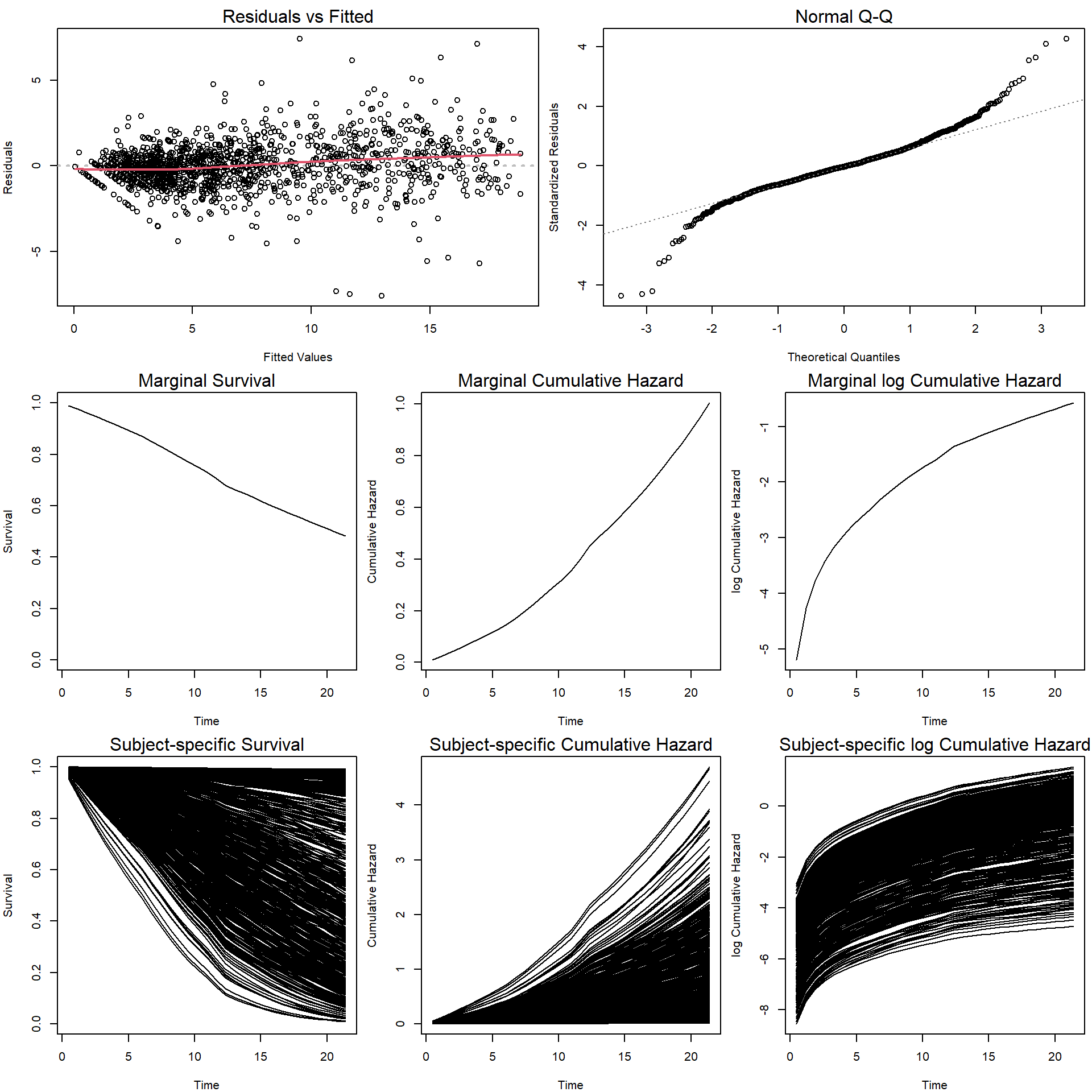 Options
 which = 6:7 should produce (cumulative) baseline
hazard, but they only work with method = "Cox-PH-GH".
par(mfrow = c(1,2))
plot(jointFit, which = 6:7)
But we can plot the estimated baseline hazard on our own. The result
should be a piecewise constant function, estimates for which are
contained inside jointFit$coefficients$xi.
par(mfrow = c(1,2), mar = c(4,4.1,2,0.5))

# Baseline hazard
plot(0, 0, type = "n", main = "Baseline hazard",
     xlab = "Time", ylab = expression(Hazard*" "*xi[k]),
     xlim = range(breaks), ylim = c(0, max(jointFit$coefficients$xi)))
segments(x0 = breaks[-length(breaks)], x1 = breaks[-1],
         y0 = jointFit$coefficients$xi, col = "saddlebrown", lwd = 2)

# Cumulative baseline hazard
cumxi <- cumsum(jointFit$coefficients$xi * diff(breaks))
plot(0, 0, type = "n", main = "Cumulative baseline hazard",
     xlab = "Time", ylab = "Cumulative Hazard",
     xlim = range(breaks), ylim = c(0, max(cumxi)))
abline(v = breaks, col = "grey", lty = 2, lwd = 0.5)
lines(breaks, c(0, cumxi), col = "saddlebrown", lwd = 2)
Function predict predicts values for the longitudinal
part of a joint model. By default it predicts the value for 25 equally
spaced time points after the last available measurement provided in
newdata.
pats <- c(1, 6, 141, 189)
(newdata <- aids[aids$patient %in% pats, ])
## patient Time death CD4 obstime drug gender prevOI AZT start stop event
## 1 1 16.97 0 10.677078 0 ddC male AIDS intolerance 0 6.00 0
## 2 1 16.97 0 8.426150 6 ddC male AIDS intolerance 6 12.00 0
## 3 1 16.97 0 9.433981 12 ddC male AIDS intolerance 12 16.97 0
## 19 6 1.90 1 4.582576 0 ddC female AIDS failure 0 1.90 1
## 410 141 10.93 1 3.162278 0 ddI male AIDS intolerance 0 2.00 0
## 411 141 10.93 1 0.000000 2 ddI male AIDS intolerance 2 6.00 0
## 412 141 10.93 1 2.236068 6 ddI male AIDS intolerance 6 10.93 1
## 571 189 1.83 0 19.235384 0 ddI male AIDS intolerance 0 1.83 0pred <- predict(jointFit, newdata = newdata, type = "Subject", interval = "prediction", idVar = "patient")
par(mfrow = c(1,length(pats)), mar = c(4,4,2,0.5))
for(i in 1:length(pats)){
subnd <- newdata[newdata$patient == pats[i],]
plot(CD4 ~ obstime, data = subnd,
xlab = "Time", ylab = "CD4", main = paste("Patient", pats[i]),
xlim = range(breaks), ylim = c(0, max(pred$upp)),
col = "royalblue", bg = "skyblue", pch = 21, cex = 1.5)
lines(attr(pred,"time.to.pred")[[i]], pred$pred[1:25 + (i-1)*25], col = "red", lwd = 2)
lines(attr(pred,"time.to.pred")[[i]], pred$low[1:25 + (i-1)*25], col = "orange", lty = 2)
lines(attr(pred,"time.to.pred")[[i]], pred$upp[1:25 + (i-1)*25], col = "orange", lty = 2)
}
Function survfitJM using Monte Carlo predicts the
conditional probability of surviving later times than the last observed
time for which a longitudinal measurement was available:
surv <- JM::survfitJM(jointFit, newdata = newdata, idVar = "patient")
par(mfrow = c(1,length(pats)), mar = c(4,4,2,0.5))
plot(surv)
Survival prediction for two patients newly incoming to the study, two different drugs given:
ND <- data.frame(patient = c(1001,1002),
                 obstime = c(0,0),
                 CD4 = c(7,7),                # average CD4 count at obstime == 0
                 drug = factor(c("ddC", "ddI")))
pred <- predict(jointFit, newdata = ND, type = "Subject", interval = "prediction", idVar = "patient")
surv <- JM::survfitJM(jointFit, newdata = ND, idVar = "patient")

par(mfrow = c(1,2), mar = c(4,4,2.5,0.5))
COL <- c("goldenrod", "royalblue")
COLlight <- c("gold", "lightblue")

# Prediction of CD4 evolution
plot(0, 0, type = "n",
     xlim = range(breaks), ylim = c(0, max(pred$upp)),
     xlab = "Time", ylab = "CD4", main = "Longitudinal prediction")
points(0, 7, col = "black", bg = "grey", pch = 21, cex = 1.5)
for(i in 1:2){
  lines(attr(pred,"time.to.pred")[[i]], pred$pred[1:25 + (i-1)*25], col = COL[i], lwd = 2)
  lines(attr(pred,"time.to.pred")[[i]], pred$low[1:25 + (i-1)*25], col = COLlight[i], lty = 2)
  lines(attr(pred,"time.to.pred")[[i]], pred$upp[1:25 + (i-1)*25], col = COLlight[i], lty = 2)
}
legend("right", levels(ND$drug), bty = "n", title = "Drug", col = COL, lty = 1, lwd = 2)

# Prediction of survival
plot(0, 0, type = "n",
     xlim = range(breaks), ylim = c(0, 1),
     xlab = "Time", ylab = "Survival probability", main = "Survival prediction")
points(0, 1, col = "black", bg = "grey", pch = 21, cex = 1.5)
for(i in 1:2){
  lines(Mean ~ times, data = surv$summaries[[i]], col = COL[i], lwd = 2)
  lines(Lower ~ times, data = surv$summaries[[i]], col = COLlight[i], lty = 2)
  lines(Upper ~ times, data = surv$summaries[[i]], col = COLlight[i], lty = 2)
}
legend("bottomleft", levels(ND$drug), bty = "n", title = "Drug", col = COL, lty = 1, lwd = 2)
Bayesian approach
The Bayesian approach is fitted in a similar way. However, it differs
in the parametrization and specification of the baseline hazard. See
Details of help(jointModelBayes) to learn what different
parametrizations of the effect of the modelled longitudinal outcome are
on the hazard with option param. The default choice
corresponds to our parametrization above. The log-baseline hazard is
modelled only by B-splines (penalized version by prior), see
baseHaz option. The knots and order of the
spline (ordSpline) are set up in the list
control. It also contains adapt,
n.iter, n.burnin, n.thin and
n.adapt to define the length of Markov chains. The list
priors specifies the hyperparameters for prior
distributions. The list init contains the initial values
for starting the Markov chains.
library(JMbayes)
library(HDInterval)
jointFitB <- jointModelBayes(lmeFit, coxFit, timeVar = "obstime")
Now we examine the contents of this object:
jointFitB##
## Call:
## jointModelBayes(lmeObject = lmeFit, survObject = coxFit, timeVar = "obstime")
##
## Variance Components:
## $`Random-Effects`
## StdDev Corr
## (Intercept) 4.5939
## obstime 0.5741 -0.0289
##
## $`Residual Std. Err.`
## sigma
## 1.7188
##
##
## Coefficients:
## $`Longitudinal Process`
## (Intercept) obstime obstime:drugddI
## 7.1903 -0.2317 0.0088
##
## $`Event Process`
## drugddI Assoct Bs.gammas1 Bs.gammas2 Bs.gammas3 Bs.gammas4 Bs.gammas5 Bs.gammas6
## 0.3296 -0.2965 -2.8036 -2.7127 -2.6391 -2.5823 -2.5386 -2.4965
## Bs.gammas7 Bs.gammas8 Bs.gammas9 Bs.gammas10 Bs.gammas11 Bs.gammas12 Bs.gammas13 Bs.gammas14
## -2.4516 -2.4133 -2.3871 -2.3891 -2.4101 -2.4401 -2.4748 -2.5083
## Bs.gammas15 Bs.gammas16 Bs.gammas17
## -2.5427 -2.5777 -2.6123
##
##
## DIC: 474139.7class(jointFitB) # JMbayes## [1] "JMbayes"jointFitB$priors$priorMean.betas # hyperparameters of prior distributions## [1] 0 0 0jointFitB$control$n.iter # total number of iterations sampled## [1] 20000jointFitB$control$n.burnin # the length of the burn-in phase## [1] 3000jointFitB$control$n.thin # thinning## [1] 10jointFitB$control$knots # knots for the spline basis ## [1] 0.002007988 0.002007988 0.002007988 0.002007988 3.771214286 4.963428571 6.155642857
## [8] 7.347857143 8.540071429 9.732285714 10.924500000 12.116714286 13.308928571 14.501142857
## [15] 15.693357143 16.885571429 18.077785714 21.400000000 21.400000000 21.400000000 21.400000000jointFitB$control$ordSpline # order of the spline basis for baseline hazard## [1] 4jointFitB$control$seed # this is where you set up the seed## [1] 1jointFitB$postMeans$betas # posterior Mean estimates## (Intercept) obstime obstime:drugddI
## 7.190337630 -0.231668241 0.008831915jointFitB$postModes$gammas # posterior Mode estimates## drugddI
## 0.3490291jointFitB$StErr$Bs.gammas # Standard Errors estimates ## Bs.gammas1 Bs.gammas2 Bs.gammas3 Bs.gammas4 Bs.gammas5 Bs.gammas6 Bs.gammas7 Bs.gammas8
## 0.01829073 0.01476564 0.01306868 0.01217552 0.01160458 0.01218013 0.01204375 0.01228668
## Bs.gammas9 Bs.gammas10 Bs.gammas11 Bs.gammas12 Bs.gammas13 Bs.gammas14 Bs.gammas15 Bs.gammas16
## 0.01251894 0.01312726 0.01445770 0.01588205 0.01666955 0.02161833 0.02635513 0.03316437
## Bs.gammas17
## 0.04105986jointFitB$CIs$alphas # ET credible intervals (95 % by default)## Assoct
## 2.5% -0.3833265
## 97.5% -0.2188212jointFitB$Pvalues # Bayesian analogy of p-value through ET CI## $betas
## [1] 0.000 0.000 0.877
##
## $sigma
## [1] 0
##
## $D
## [1] 0.000 0.604 0.604 0.000
##
## $gammas
## [1] 0.095
##
## $Bs.gammas
## [1] 0 0 0 0 0 0 0 0 0 0 0 0 0 0 0 0 0
##
## $tauBs
## [1] 0
##
## $alphas
## [1] 0# jointFitB$vcov # Variance-covariance matrix among all model parameters
head(jointFitB$mcmc$D) # sampled chains## D[1, 1] D[2, 1] D[1, 2] D[2, 2]
## [1,] 19.87876 0.03836447 0.03836447 0.2996788
## [2,] 22.13644 -0.09128929 -0.09128929 0.3209435
## [3,] 20.74985 0.04069021 0.04069021 0.2889551
## [4,] 22.49089 -0.13321169 -0.13321169 0.3710575
## [5,] 20.36252 -0.10407358 -0.10407358 0.2866503
## [6,] 20.43969 -0.02503158 -0.02503158 0.2987289lapply(jointFitB$mcmc, hdi) # Highest Posterior Density Credible Intervals, library(HDInterval)## $betas
## (Intercept) obstime obstime:drugddI
## lower 6.762409 -0.3142609 -0.1111266
## upper 7.613233 -0.1419485 0.1348963
## attr(,"credMass")
## [1] 0.95
##
## $sigma
## sigma
## lower 1.619126
## upper 1.819198
## attr(,"credMass")
## [1] 0.95
##
## $b
## lower upper
## -6.381354 8.131627
## attr(,"credMass")
## [1] 0.95
##
## $D
## D[1, 1] D[2, 1] D[1, 2] D[2, 2]
## lower 18.20064 -0.3793769 -0.3793769 0.2726199
## upper 24.13217 0.2300917 0.2300917 0.3861688
## attr(,"credMass")
## [1] 0.95
##
## $gammas
## drugddI
## lower -0.03787297
## upper 0.70092450
## attr(,"credMass")
## [1] 0.95
##
## $Bs.gammas
## Bs.gammas1 Bs.gammas2 Bs.gammas3 Bs.gammas4 Bs.gammas5 Bs.gammas6 Bs.gammas7 Bs.gammas8
## lower -3.338865 -3.135212 -3.021408 -2.900799 -2.845472 -2.832086 -2.776659 -2.753314
## upper -2.268921 -2.292135 -2.279775 -2.225913 -2.190104 -2.169244 -2.129408 -2.085837
## Bs.gammas9 Bs.gammas10 Bs.gammas11 Bs.gammas12 Bs.gammas13 Bs.gammas14 Bs.gammas15
## lower -2.718079 -2.733021 -2.778234 -2.793933 -2.942410 -3.020425 -3.201066
## upper -2.043946 -2.040454 -2.021664 -1.980983 -2.008022 -1.950891 -1.878983
## Bs.gammas16 Bs.gammas17
## lower -3.444652 -3.764131
## upper -1.762172 -1.616662
## attr(,"credMass")
## [1] 0.95
##
## $tauBs
## tauBs
## lower 38.3158
## upper 846.4514
## attr(,"credMass")
## [1] 0.95
##
## $alphas
## Assoct
## lower -0.3806329
## upper -0.2180476
## attr(,"credMass")
## [1] 0.95jointFitB$DIC # Deviance Information Criterion## [1] 474139.7The outputs of traditional functions resemble the outputs for MLE approach:
summary(jointFitB)##
## Call:
## jointModelBayes(lmeObject = lmeFit, survObject = coxFit, timeVar = "obstime")
##
## Data Descriptives:
## Longitudinal Process Event Process
## Number of Observations: 1405 Number of Events: 188 (40.3%)
## Number of subjects: 467
##
## Joint Model Summary:
## Longitudinal Process: Linear mixed-effects model
## Event Process: Relative risk model with penalized-spline-approximated
## baseline risk function
## Parameterization: Time-dependent value
##
## LPML DIC pD
## -Inf 474139.7 232406.1
##
## Variance Components:
## StdDev Corr
## (Intercept) 4.5939 (Intr)
## obstime 0.5741 -0.0289
## Residual 1.7188
##
## Coefficients:
## Longitudinal Process
## Value Std.Err Std.Dev 2.5% 97.5% P
## (Intercept) 7.1903 0.0054 0.2200 6.7519 7.6088 <0.001
## obstime -0.2317 0.0012 0.0444 -0.3204 -0.1469 <0.001
## obstime:drugddI 0.0088 0.0018 0.0629 -0.1111 0.1349 0.877
##
## Event Process
## Value Std.Err Std.Dev 2.5% 97.5% P
## drugddI 0.3296 0.0102 0.1978 -0.0726 0.6783 0.095
## Assoct -0.2965 0.0021 0.0426 -0.3833 -0.2188 <0.001
## tauBs 381.6132 18.8686 252.9150 67.6810 1011.4651 NA
##
## MCMC summary:
## iterations: 20000
## adapt: 3000
## burn-in: 3000
## thinning: 10
## time: 1.1 minfixef(jointFitB)## (Intercept) obstime obstime:drugddI
## 7.190337630 -0.231668241 0.008831915head(coef(jointFitB, "Longitudinal"))## (Intercept) obstime obstime:drugddI
## [1,] 9.871951 -0.1420444 0.008831915
## [2,] 7.091661 -0.2092840 0.008831915
## [3,] 4.598255 -0.1455689 0.008831915
## [4,] 4.445164 -0.2804179 0.008831915
## [5,] 8.219124 -0.1739527 0.008831915
## [6,] 4.150560 -0.4316105 0.008831915coef(jointFitB, "Event")## drugddI Assoct
## 0.3295682 -0.2964958confint(jointFitB)## 2.5 % est. 97.5 %
## Y.(Intercept) 6.75194914 7.190337630 7.6087813
## Y.obstime -0.32039245 -0.231668241 -0.1469199
## Y.obstime:drugddI -0.11112864 0.008831915 0.1348872
## T.drugddI -0.07262605 0.329568205 0.6783042
## T.Assoct -0.38332653 -0.296495759 -0.2188212# anova(jointFitB) # only works for two models
# logLik(jointFitB) # why error? The residual plots by plot are now in
plot.JMbayes replaced with traceplots, autocorrelation
functions and density estimates (in a window \(2\times 2\)).
plot(jointFitB, which = "trace", param = c("betas", "gammas"))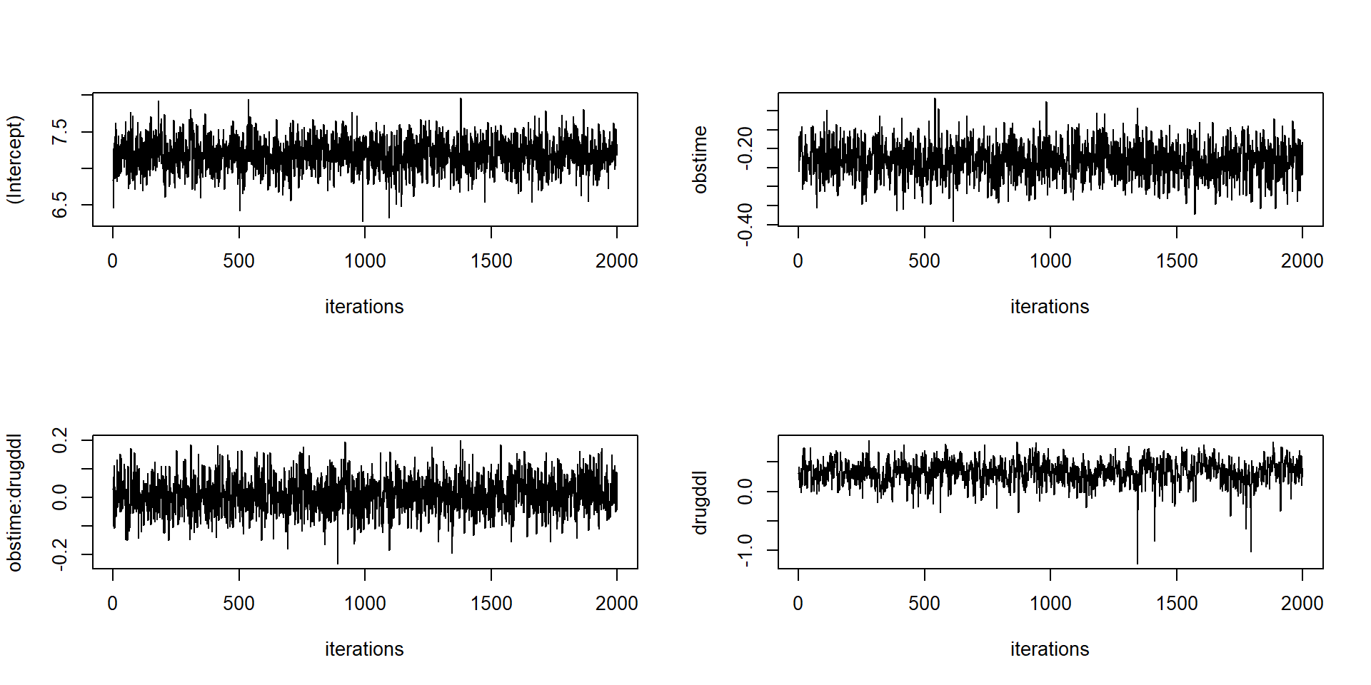
plot(jointFitB, which = "autocorr", param = c("sigma", "D"))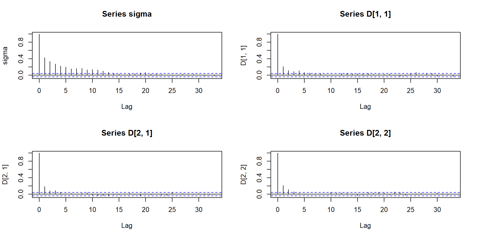
plot(jointFitB, which = "density", param = c("alphas", "betas"))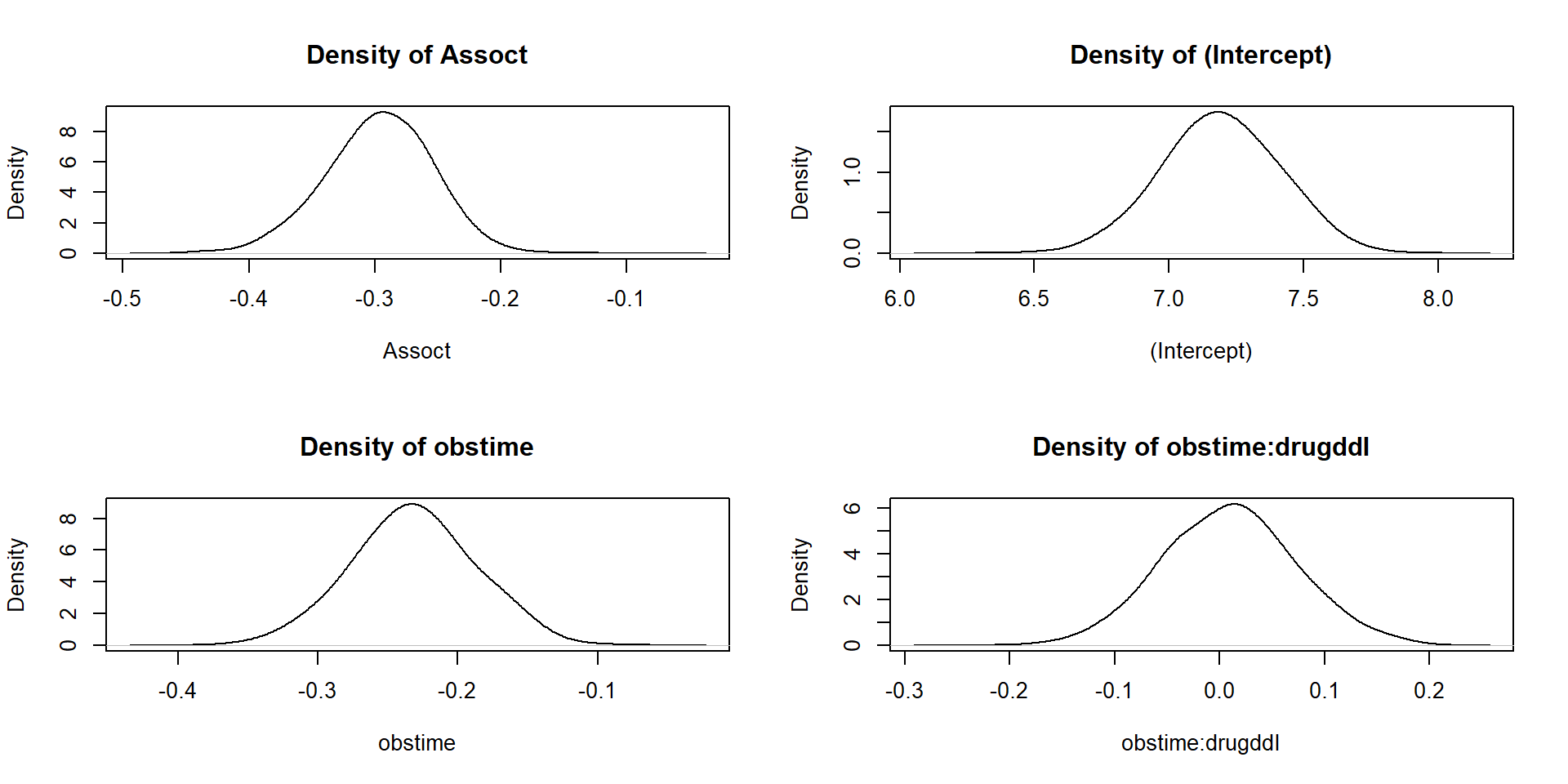
There is no function for plotting the posterior distribution of the baseline hazard function estimated by splines. We have to explore it on our own:
library(splines)
jointFitB$baseHaz                               # only information about type of splines
## [1] "P-splines"tgrid <- seq(0, 20, length.out = 101)[-1]
ncoefs <- dim(jointFitB$mcmc$Bs.gammas)[2]
ord <- jointFitB$control$ordSpline
knots <- unique(jointFitB$control$knots)
BSB <- bs(tgrid, degree = ord,
knots = knots[-c(1,length(knots))],
Boundary.knots = knots[c(1,length(knots))])
ncoefs == dim(BSB)[2] # great, the number of coefficients matches!## [1] TRUEbasehaz <- exp(jointFitB$mcmc$Bs.gammas %*% t(BSB))
basehaz_post <- t(apply(basehaz, 2, function(x){
c(quantile(x, probs = 0.025), mean(x), quantile(x, probs = 0.975))
}))
cumbasehaz <- t(apply(basehaz, 1, function(h){
# we need cumulative approximation of the integral
# integral between t1 < t2 with values h(t1) and h(t2) is approximated by
# (h(t1) + h(t2))/2 * (t2 - t1)
avg_neighbours <- zoo::rollmean(c(0,h), 2)
diff_time <- diff(c(0, tgrid))
ret <- cumsum(avg_neighbours * diff_time)
return(ret)
}))
cumbasehaz_post <- t(apply(cumbasehaz, 2, function(x){
c(quantile(x, probs = 0.025), mean(x), quantile(x, probs = 0.975))
}))
par(mfrow = c(1,2), mar = c(4,4,2.5,1))
# Baseline hazard
plot(tgrid, basehaz_post[,2], xlim = c(0, max(breaks)), ylim = c(0.05, 0.15),
type = "l", col = "saddlebrown", lwd = 2,
xlab = "Time", ylab = "Hazard", main = "Baseline hazard")
lines(tgrid, basehaz_post[,1], col = "goldenrod", lty = 2)
lines(tgrid, basehaz_post[,3], col = "goldenrod", lty = 2)
legend("top", c("Posterior Mean", "ET CI 95 %"), bty = "n", ncol = 2,
col = c("saddlebrown", "goldenrod"), lwd = c(2,1), lty = c(1,2))
# Cumulative baseline hazard
plot(c(0,tgrid), c(0, cumbasehaz_post[,2]), xlim = c(0, max(breaks)), ylim = c(0, 2),
type = "l", col = "saddlebrown", lwd = 2,
xlab = "Time", ylab = "Hazard", main = "Cumulative baseline hazard")
lines(c(0,tgrid), c(0, cumbasehaz_post[,1]), col = "goldenrod", lty = 2)
lines(c(0,tgrid), c(0, cumbasehaz_post[,3]), col = "goldenrod", lty = 2)
legend("topleft", c("Posterior Mean", "ET CI 95 %"), bty = "n",
col = c("saddlebrown", "goldenrod"), lwd = c(2,1), lty = c(1,2)) The high baseline hazard for low values of time is probably due to much
higher proportion of deaths occurring within the first 2 months:
The high baseline hazard for low values of time is probably due to much
higher proportion of deaths occurring within the first 2 months:
aids[aids$Time <= 2, ] # almost all have event = death = 1## patient Time death CD4 obstime drug gender prevOI AZT start stop event
## 19 6 1.90 1 4.582576 0 ddC female AIDS failure 0 1.90 1
## 134 49 2.00 1 1.000000 0 ddI male noAIDS intolerance 0 2.00 1
## 190 69 0.77 1 2.236068 0 ddC male AIDS failure 0 0.77 1
## 200 73 1.30 1 1.000000 0 ddI male AIDS intolerance 0 1.30 1
## 318 108 1.07 1 1.414214 0 ddC male AIDS failure 0 1.07 1
## 571 189 1.83 0 19.235384 0 ddI male AIDS intolerance 0 1.83 0
## 594 196 1.70 1 4.472136 0 ddI male AIDS intolerance 0 1.70 1
## 889 292 1.43 1 1.732051 0 ddC female AIDS intolerance 0 1.43 1
## 1030 337 1.13 1 3.464102 0 ddI female AIDS failure 0 1.13 1
## 1054 344 1.07 1 2.236068 0 ddC male AIDS intolerance 0 1.07 1
## 1086 355 0.47 1 18.466185 0 ddI female noAIDS intolerance 0 0.47 1
## 1141 376 1.63 1 0.000000 0 ddI male AIDS failure 0 1.63 1
## 1251 415 1.03 1 2.000000 0 ddC male AIDS intolerance 0 1.03 1
## 1282 427 1.43 1 6.000000 0 ddC male AIDS failure 0 1.43 1
## 1367 453 0.90 1 6.324555 0 ddI female AIDS failure 0 0.90 1
## 1401 464 2.00 1 4.898979 0 ddC male AIDS intolerance 0 2.00 1Function predict predicts values for the longitudinal
part of a joint model. Its syntax is analogical to the one in MLE
approach.
pats <- c(1, 6, 141, 189)
(newdata <- aids[aids$patient %in% pats, ])
## patient Time death CD4 obstime drug gender prevOI AZT start stop event
## 1 1 16.97 0 10.677078 0 ddC male AIDS intolerance 0 6.00 0
## 2 1 16.97 0 8.426150 6 ddC male AIDS intolerance 6 12.00 0
## 3 1 16.97 0 9.433981 12 ddC male AIDS intolerance 12 16.97 0
## 19 6 1.90 1 4.582576 0 ddC female AIDS failure 0 1.90 1
## 410 141 10.93 1 3.162278 0 ddI male AIDS intolerance 0 2.00 0
## 411 141 10.93 1 0.000000 2 ddI male AIDS intolerance 2 6.00 0
## 412 141 10.93 1 2.236068 6 ddI male AIDS intolerance 6 10.93 1
## 571 189 1.83 0 19.235384 0 ddI male AIDS intolerance 0 1.83 0pred <- predict(jointFitB, newdata = newdata, type = "Subject", interval = "confidence", idVar = "patient")
par(mfrow = c(1,length(pats)), mar = c(4,4,2,0.5))
for(i in 1:length(pats)){
subnd <- newdata[newdata$patient == pats[i],]
plot(CD4 ~ obstime, data = subnd,
xlab = "Time", ylab = "CD4", main = paste("Patient", pats[i]),
xlim = range(breaks), ylim = c(0, max(aids$CD4)),
col = "royalblue", bg = "skyblue", pch = 21, cex = 1.5)
lines(attr(pred,"time.to.pred")[[i]], pred$pred[1:25 + (i-1)*25], col = "red", lwd = 2)
lines(attr(pred,"time.to.pred")[[i]], pred$low[1:25 + (i-1)*25], col = "orange", lty = 2)
lines(attr(pred,"time.to.pred")[[i]], pred$upp[1:25 + (i-1)*25], col = "orange", lty = 2)
}
Function survfitJM using Monte Carlo predicts the
conditional probability of surviving later times than the last observed
time for which a longitudinal measurement was available:
surv <- survfitJM(jointFitB, newdata = newdata, idVar = "patient")
par(mfrow = c(1,length(pats)), mar = c(4,4,2,0.5))
plot(surv)
Survival prediction for two patients newly incoming to the study, two different drugs given:
ND <- data.frame(patient = c(1001,1002),
                 obstime = c(0,0),
                 CD4 = c(7,7),                # average CD4 count at obstime == 0
                 drug = factor(c("ddC", "ddI")))
pred <- predict(jointFitB, newdata = ND, type = "Subject", interval = "prediction", idVar = "patient")
surv <- survfitJM(jointFitB, newdata = ND, idVar = "patient")

par(mfrow = c(1,2), mar = c(4,4,2.5,0.5))
COL <- c("goldenrod", "royalblue")
COLlight <- c("gold", "lightblue")

# Prediction of CD4 evolution
plot(0, 0, type = "n",
     xlim = range(breaks), ylim = c(0, max(pred$upp)),
     xlab = "Time", ylab = "CD4", main = "Longitudinal prediction")
points(0, 7, col = "black", bg = "grey", pch = 21, cex = 1.5)
for(i in 1:2){
  lines(attr(pred,"time.to.pred")[[i]], pred$pred[1:25 + (i-1)*25], col = COL[i], lwd = 2)
  lines(attr(pred,"time.to.pred")[[i]], pred$low[1:25 + (i-1)*25], col = COLlight[i], lty = 2)
  lines(attr(pred,"time.to.pred")[[i]], pred$upp[1:25 + (i-1)*25], col = COLlight[i], lty = 2)
}
legend("right", levels(ND$drug), bty = "n", title = "Drug", col = COL, lty = 1, lwd = 2)

# Prediction of survival
plot(0, 0, type = "n",
     xlim = range(breaks), ylim = c(0, 1),
     xlab = "Time", ylab = "Survival probability", main = "Survival prediction")
points(0, 1, col = "black", bg = "grey", pch = 21, cex = 1.5)
for(i in 1:2){
  lines(Mean ~ times, data = surv$summaries[[i]], col = COL[i], lwd = 2)
  lines(Lower ~ times, data = surv$summaries[[i]], col = COLlight[i], lty = 2)
  lines(Upper ~ times, data = surv$summaries[[i]], col = COLlight[i], lty = 2)
}
legend("bottomleft", levels(ND$drug), bty = "n", title = "Drug", col = COL, lty = 1, lwd = 2)