Testing equality of censored distributions
Jan Vávra
Exercise 5 (30th November - 7th December 2020)
Theory
The two-sample problem in censored data analysis
We consider two independent censored samples of sizes \(n_1\) and \(n_2\), one sample with survival function \(S_1(t)\) and cumulative hazard \(\Lambda_1(t)\), the other sample with survival function \(S_2(t)\) and cumulative hazard \(\Lambda_2(t)\). The censoring distribution need not be the same in both groups.
Consider the hypothesis \[ \begin{aligned} \mathrm{H}_0: &\, S_1(t)=S_2(t) \quad \forall t>0, \\ \mathrm{H}_1: &\, S_1(t)\neq S_2(t) \quad \text{ for some } t>0, \end{aligned} \quad \Longleftrightarrow \quad \begin{aligned} \mathrm{H}_0: &\, \Lambda_1(t)=\Lambda_2(t) \quad \forall t>0, \\ \mathrm{H}_1: &\, \Lambda_1(t)\neq \Lambda_2(t) \quad \text{ for some } t>0. \end{aligned} \]
Weighted logrank statistics
The class of weighted logrank test statistics for testing \(H_0\) against \(H_1\) is \[ W_K=\int_0^\infty K(s)\,\mathrm{d}(\widehat{\Lambda}_1-\widehat{\Lambda}_2)(s), \] where \[ K(s)=\sqrt{\frac{n_1n_2}{n_1+n_2}} \frac{\overline{Y}_1(s)}{n_1}\, \frac{\overline{Y}_2(s)}{n_2}\,\frac{n_1+n_2}{\overline{Y}(s)}W(s) \] and \(W(s)\) is a weight function – it governs the power of the test against different alternatives.
\(W(s)=1\) is the logrank test. It is most powerful against proportional hazards alternatives, i.e., \(\lambda_1(t)=c\lambda_2(t)\) for some positive constant \(c\neq 1\).
\(W(s)=\overline{Y}(s)/(n+1)\) is the Gehan-Wilcoxon test which in the uncensored case is equivalent to two-sample Wilcoxon test. This test puts more weight on early differences in hazard functions than on differences that occur later.
\(W(s)=\widehat{S}(s-)\) is the Prentice-Wilcoxon test (also known as Peto-Prentice or Peto and Peto test). It is especially powerful against alternatives with strong early effects that weaken over time. Preferred compared to Gehan-Wilcoxon test.
\(W(s)=\left[\widehat{S}(s-)\right]^\rho\left[1-\widehat{S}(s-)\right]^\gamma\) is the \(G(\rho,\gamma)\) class of tests of Fleming-Harrington. The logrank test is a special case for \(\rho=\gamma=0\), the Prentice-Wilcoxon test is a special case for \(\rho=1,\ \gamma=0\). The \(G(0,1)\) test is especially powerful against alternatives with little initial difference in hazards that gets stronger over time.
Let \(\widehat\sigma^2_K\) be the estimated variance of \(W_K\) under \(H_0\), which is of the form \[ \widehat{\sigma}_K^2 = \int \limits_{0}^{\infty} \dfrac{K^2(s)}{\overline{Y}_1(s) \overline{Y}_2(s)} \left(1 - \dfrac{\Delta \overline{N}(s)-1}{\overline{Y}(s) - 1}\right) \,\mathrm{d} \overline{N}(s). \] It can be shown that, under \(H_0\), \[ \frac{W_K}{\widehat\sigma_K}\stackrel{D}{\longrightarrow}\mathsf{N}(0,1) \qquad\text{ and }\qquad \frac{W^2_K}{\widehat\sigma^2_K}\stackrel{D}{\longrightarrow}\chi^2_1. \]
Calculation of weighted logrank statistics
Let \(t_1<t_2<\cdots<t_d\) be the ordered distinct failure times in both samples. The weighted logrank test statistic (without the normalizing constant depending on \(n_1\) and \(n_2\)) can be written as \[ \sum_{j=1}^d \biggl(\Delta\overline{N}_1(t_j)-\Delta\overline{N}(t_j) \frac{\overline{Y_1}(t_j)}{\overline{Y}(t_j)}\biggr) W(t_j). \] The variance estimator \(\widehat{\sigma}_K^2\) (again without the normalizing constant depending on \(n_1\) and \(n_2\)) can be calculated using the following formula \[ \sum \limits_{j = 1}^d \Delta N(t_j) \cdot \dfrac{\overline{Y}_1(t_j) \overline{Y}_2(t_j)}{\left(\overline{Y}(t_j)\right)^2} \cdot \dfrac{\overline{Y}(t_j) - \Delta N(t_j)}{\overline{Y}(t_j) - 1} \cdot \left(W(t_j)\right)^2. \]
Download the dataset km_all.RData.
The dataframe inside is called all. It includes 101 observations and three variables. The observations are acute lymphatic leukemia [ALL] patients who had undergone bone marrow transplant. The variable time contains time (in months) since transplantation to either death/relapse or end of follow up, whichever occured first. The outcome of interest is time to death or relapse of ALL (relapse-free survival). The variable delta includes the event indicator (1 = death or relapse, 0 = censoring). The variable type distinguishes two different types of transplant (1 = allogeneic, 2 = autologous).
Using ordinary R functions (not the survival library), calculate and print the following table:
| \(j\) | \(t_j\) | \(d_{1j}\) | \(d_{j}\) | \(y_{1j}\) | \(y_j\) | \(e_j=d_j\frac{y_{1j}}{y_j}\) | \(d_{1j}-e_j\) | \(v_j=d_j\dfrac{y_{1j} (y_j-y_{1j}) (y_j-d_j)}{y_j^2 (y_j - 1)}\) |
|---|---|---|---|---|---|---|---|---|
| 1 | … | … | … | … | … | … | … | … |
| … | … | … | … | … | … | … | … | … |
| d | … | … | … | … | … | … | … | … |
where \(j\) is the order of the failures, \(t_j\) is the ordered failure time, \(d_{1j}=\Delta\overline{N}_1(t_j)\), \(d_j=\Delta\overline{N}(t_j)\), \(y_{1j}=\overline{Y}_1(t_j)\), \(y_j=\overline{Y}(t_j)\).
Use these values to perform logrank test on your own.
BONUS: Try to implement \(G(\rho,\gamma)\) test, remember, you need left-continuous version of Kaplan-Meier estimator of survival function.
Implementation in R
The function survdiff in the library survival can calculate \(G(\rho,0)\) statistics. The default is \(\rho=0\), that is, the logrank test. Output is a list with:
$chisq- test statistic in the squared form \(W_K^2/\widehat{\sigma}_K^2\),$var[1,1]- variance estimator \(\widehat{\sigma}_K^2\),- no p-value stored, you need to get it manually by
pchisq(...$chisq, df=1, lower.tail = F).
library(survival)
survdiff(Surv(time,delta)~type,data=all)
survdiff(Surv(time,delta)~type,data=all,rho=2)
## Call:
## survdiff(formula = Surv(time, delta) ~ type, data = all)
##
## N Observed Expected (O-E)^2/E (O-E)^2/V
## type=1 50 22 24.2 0.195 0.382
## type=2 51 28 25.8 0.182 0.382
##
## Chisq= 0.4 on 1 degrees of freedom, p= 0.5The function FHtestrcc in the library FHtest can calculate \(G(\rho,\gamma)\) statistics for non-zero \(\gamma\). The default is \(\rho=0,\ \gamma=0\), that is, the logrank test. The parameter \(\gamma\) is entered as the argument lambda. For the proper choice of \(\rho\) and \(\gamma\) read Details of help(FHtestrcc). Output is a list with:
$statistic- test statistic in the form \(W_K/\widehat{\sigma}_K\),$var- variance estimator \(\widehat{\sigma}_K^2\),$pvalue- pvalue of the test associated with the selected alternative hypothesis (parameteralternative),- …
library(FHtest)
FHtestrcc(Surv(time,delta)~type, data=all)
FHtestrcc(Surv(time,delta)~type, data=all, rho=0.5, lambda=2)
##
## Two-sample test for right-censored data
##
## Parameters: rho=0.5, lambda=2
## Distribution: counting process approach
##
## Data: Surv(time, delta) by type
##
## N Observed Expected O-E (O-E)^2/E (O-E)^2/V
## type=1 50 0.961 1.69 -0.732 0.316 5.63
## type=2 51 2.369 1.64 0.732 0.327 5.63
##
## Statistic Z= 2.4, p-value= 0.0176
## Alternative hypothesis: survival functions not equalCaution
The library FHtest requires library Icens which has been removed from R and cannot be installed by standard methods. It is available from the Bioconductor repository. It can be downloaded manually and installed by a command such as:
install.packages("http://www.karlin.mff.cuni.cz/~vavraj/cda/data/Icens_1.38.0.zip", repos =NULL)survdiff and FHtestrcc output)
Compare your calculation of logrank test with the output of the functions survdiff and FHtestrcc in the case of dataset all.
In the all data, investigate the difference in survival and hazard functions according to the type of transplant. Remember that the outcome is relapse-free survival.
Calculate and plot estimated survival functions by the type of transplant (1 = allogeneic, 2 = autologous). Distinguish the groups by color. Add a legend.
Calculate and plot Nelson-Aalen estimators of cumulative hazard functions by the type of transplant (1 = allogeneic, 2 = autologous). Distinguish the groups by color. Add a legend.
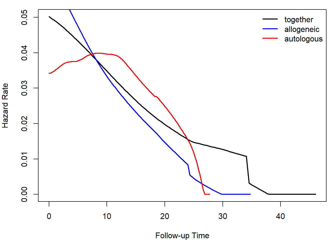
Calculate and plot smoothed hazard functions by the type of transplant (1 = allogeneic, 2 = autologous). Distinguish the groups by color. Add a legend.
Perform logrank, Prentice-Wilcoxon and \(G(0,1)\) tests using functions
survdifforFHtestrcc. Interpret the results. Which test is more suitable in this case?
- Deadline: Monday 7th December 9:00.
Hint for obtaining smoothed hazard functions:
library(muhaz)
haz = muhaz(all$time,all$delta)
plot(haz, col = "black", lwd = 2)