Actuarial (lifetable) estimator of the survival

Lifetable or actuarial estimator

Applies when the data are grouped

Our goal is still to estimate the survival function, hazard, and density function, but this is complicated by the fact that we don’t know exactly when during each time interval an event occurs.

Notation:

the $j$ -th time interval is $[t_{j-1},t_j)$ ,
$c_j$ - the number of censorings in the $j$ -th interval,
$d_j$ - the number of failures (deaths) in the $j$ -th interval,
$r_j$ - the number of units entering the interval.

We could apply the K-M formula directly. However, this approach is unsatisfactory for grouped data … it treats the problem as though it were in discrete time, with events happening only at 1 yr, 2 yr, etc. In fact, what we are trying to calculate here is the conditional probability of dying within the interval, given survival to the beginning of it.

We now make the assumption that the censoring process is such that the censored survival times occur uniformly throughout the $j$ -th interval. So, we can assume that censorings occur on average halfway through the interval: $r_j'=r_j-c_j/2.$ I.e., average number of individuals who are at risk during this interval. The assumption yields the Actuarial Estimator. It is appropriate if censorings occur uniformly throughout the interval. This assumption is sometimes known as the actuarial assumption.

The event that an individual survives beyond $[t_{j-1},t_j)$ is equivalent to the event that an individual survives beyond $[t_{0},t_1)$ and … and that an individual survives beyond $[t_{j-2},t_{j-1})$ and that an individual survives beyond $[t_{j-1},t_j)$ . Let us define the following quantities:

$P_j=P\{\mbox{an individual survives beyond }[t_{j-1},t_j)\}$ ,
$p_j=P\{\mbox{an individual survives beyond }[t_{j-1},t_j) |\mbox{ he survives beyond }[t_{j-2},t_{j-1})\}, \quad j>1$ ,
$p_1=P_1.$

Then by chain rule, $P_j=p_1\ldots p_j.$ The conditional probability of an death in $[t_{j-1},t_j)$ given that the individual survives beyond $[t_{j-2},t_{j-1})$ is estimated by $d_j/r_j'.$ Thus, $p_j$ is estimated by $\frac{r_j'-d_j}{r_j'}.$ So, the actuarial (lifetime) estimate of the survival function is $\widehat{S}(t)=\prod_{j=1}^{k-1}\frac{r_j'-d_j}{r_j'} \qquad \text{for } t_{k-1} \leq t < t_{k}.$

Remarks:

Because the intervals are defined as $[t_{j-1}, t_j)$ , the first interval typically starts with $t_0 = 0$ .
The implication in R is that $\widehat{S}(t_0)=1$ .

The form of the estimated survivor function obtained using this method is sensitive to the choice of the intervals used in its construction. On the other hand, the lifetable estimate is particularly well suited to situations in which the actual death times are unknown, and only available information is the number of deaths and the number of censored observations which occur in a series of consecutive time intervals.

Quantities estimated

Midpoint $t_{mj}=(t_j+t_{j-1})/2$ .
Width $b_j=t_j-t_{j-1}$ .
Conditional probability of dying $\widehat{q}_j=d_j/r_j'$ .
Conditional probability of surviving $\widehat{p}_j=1-\widehat{q}_j$ .
Cumulative probability of surviving at $t_j$ : $\widehat{S}(t)=\prod_{l\leq j}\widehat{p}_l$ .
Hazard in the $j$ -th interval $\widehat{\lambda}(t_{mj})=\frac{\widehat{q}_j}{b_j(1-\widehat{q}_j/2)}$ the number of deaths in the interval divided by the average number of survivors at the midpoint.
Density at the midpoint of the $j$ -th interval $\widehat{f}(t_{mj})=\frac{\widehat{S}(t_{j-1})\widehat{q}_j}{b_j}.$

Constructing the lifetable

R with KMsurv package requires three elements:

a vector of $K + 1$ interval endpoints
a $K$ vector of death counts in each interval
a $K$ vector of censored counts in each interval

Incidentally, KM in KMsurv stands for Klein and Moeschberger, not Kaplan-Meier!

library(KMsurv)

Duration of nursing home stay data

The National Center for Health Services Research studied 36 for-profit nursing homes to assess the effects of different financial incentives on length of stay. ‘Treated’ nursing homes received higher per diems for Medicaid patients, and bonuses for improving a patient’s health and sending them home.

Study included 1601 patients admitted between May 1, 1981 and April 30, 1982.

Variables include:

los - Length of stay of a resident (in days)
age - Age of a resident
rx - Nursing home assignment (1:bonuses, 0:no bonuses)
gender - Gender (1:male, 0:female)
married - (1:married, 0:not married)
health - Health status (2:second best, 5:worst)
censor - Censoring indicator (1:censored, 0:discharged)

Suppose we wish to use the actuarial method, but the data do not come grouped.

Consider the treated nursing home patients, with length of stay (los) grouped into 100 day intervals:

nurshome = read.table("http://www.karlin.mff.cuni.cz/~vavraj/cda/data/NursingHome.dat",
  head=F, skip=14, col.names = c("los", "age", "rx", "gender", "married", "health", "censor"))
nurshome$int = floor(nurshome$los/100)*100    # group in 100 day intervals
nurshome = nurshome[nurshome$rx==1,]   # keep only treated homes
nurshome[1:3,]    # check out a few observations

##    los age rx gender married health censor  int
## 1   37  86  1      0       0      2      0    0
## 2   61  77  1      0       0      4      0    0
## 3 1084  75  1      0       0      3      1 1000

tab = table(nurshome$int, nurshome$censor)
intEndpts = (0:11)*100
ntotal = dim(nurshome)[1]  # nr patients
cens = tab[,2]   # nr censored in each interval
released = tab[,1]   # nr released in each interval
fitlt = lifetab(tis = intEndpts, ninit=ntotal, nlost=cens, nevent=released)
names(fitlt)  # check out components of fitlt object

##  [1] "nsubs"     "nlost"     "nrisk"     "nevent"    "surv"      "pdf"       "hazard"    "se.surv"   "se.pdf"    "se.hazard"

round(fitlt, 5)        # restrict output to 5 decimals

##           nsubs nlost nrisk nevent    surv     pdf  hazard se.surv  se.pdf se.hazard
## 0-100       712     0 712.0    330 1.00000 0.00463 0.00603 0.00000 0.00019   0.00032
## 100-200     382     0 382.0     86 0.53652 0.00121 0.00254 0.01869 0.00012   0.00027
## 200-300     296     0 296.0     65 0.41573 0.00091 0.00247 0.01847 0.00011   0.00030
## 300-400     231     0 231.0     38 0.32444 0.00053 0.00179 0.01755 0.00008   0.00029
## 400-500     193     1 192.5     32 0.27107 0.00045 0.00181 0.01666 0.00008   0.00032
## 500-600     160     0 160.0     13 0.22601 0.00018 0.00085 0.01568 0.00005   0.00023
## 600-700     147     0 147.0     13 0.20764 0.00018 0.00093 0.01521 0.00005   0.00026
## 700-800     134    30 119.0     10 0.18928 0.00016 0.00088 0.01469 0.00005   0.00028
## 800-900      94    29  79.5      4 0.17337 0.00009 0.00052 0.01429 0.00004   0.00026
## 900-1000     61    30  46.0      4 0.16465 0.00014 0.00091 0.01422 0.00007   0.00045
## 1000-1100    27    27  13.5      0 0.15033      NA      NA 0.01468      NA        NA

Non-grouped approach

library(survival)
nurshome$delta <- 1-nurshome$censor
fit <- survfit(Surv(los,delta)~1, data = nurshome[nurshome$rx==1,])

Estimated Survival

x = rep(intEndpts, each = 2)[2:23]
y = rep(fitlt$surv, each = 2)
plot(fit, conf.int = F, col="red", xlab="Time Interval [days]", ylab="Survival probability")
lines(x, y, col="blue")
title(main = "Duration of stay in nursing homes", cex=.6)
legend("topright", c("Kaplan-Meier", "Lifetable estimator"), col = c("red", "blue"), lty = 1, bty = "n")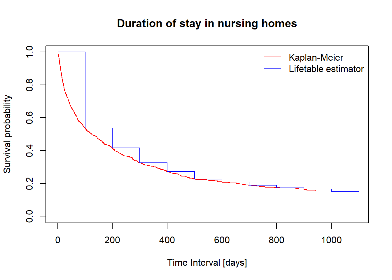

Estimated Hazard

You can use library(muhaz) to get smoothed estimator of hazard function.

y = rep(fitlt$hazard, each = 2)
library(muhaz)
haz = muhaz(nurshome$los[nurshome$rx==1],nurshome$delta[nurshome$rx==1])

plot(haz, col = "red", xlab="Time Interval [days]", ylab="Hazard")
lines(x, y, type="l", col="blue")
title(main = "Duration of stay in nursing homes", cex=.6)
legend("topright", c("Smoothed estimator", "Lifetable estimator"), col = c("red", "blue"), lty = 1, bty = "n")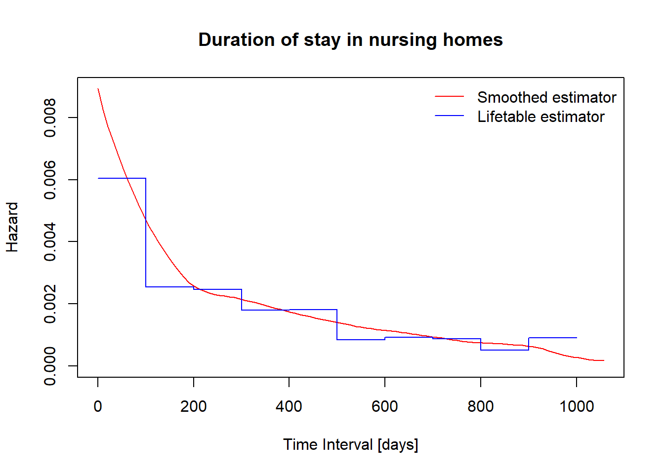

Homework assignment

Go back to the Warm-up Task with mortality datasets mort.RData. Perform actuarial estimates of survival function and hazard function and compare it with the classical Kaplan-Meier approach from the start of the lecture.

Compare your results to the official mortality tables created by ČSÚ: here for the males, here for the females. Can you recognize the columns in their table? Are their results comparable to yours? What is the cause of that in your opinion?

Include the code, output and comments in your report.

Bonus task: Could you find suitable correction of our approach, so that results are more similar to ČSÚ output? Hint: look at the given data, forget about KM approach and just think about conditional probabilities in a simple way.

Deadline for report: next exercise class 25th November

Actuarial (lifetable) estimator of the survival

Jan Vávra

Exercise 3 (18th November 2019)

Lifetable or actuarial estimator

Quantities estimated

Constructing the lifetable

Duration of nursing home stay data