Question 1 - Order of Implicit & Explicit methods

Contents

Exact solution

function q1_solution

We solve the logistic equation

$\begin{array}{rcll} x'(t) &=& (a-bx(t))x(t), &\qquad t\in[0,2], \\ x(0) &=& x_0, \end{array}$

with $a=b=1$, $x_0=2$, which has the known exact solution

$x(t) = \frac{x_0 e^t}{1-x_0(1-e^t)}.$

x0 = 2;
timepoint = 2;
exact = x0*exp(timepoint)/(1-x0*(1-exp(timepoint)));
no_approx = 10;
h = 0.5.^(1:no_approx)';

Euler

error = zeros(no_approx,1);
for ei=1:no_approx
  x = solve(@eul, @logistic, 0, 2, x0, h(ei), timepoint);
  error(ei) = norm(exact-x);
end
[p,q]=regrese(h,error);

figure;
plot(h,error,'-ro');
title('Euler');
xlabel('\tau');
ylabel('error');

figure;
loglog(h,error,'-ro');
title('Euler')
xlabel('\tau');
ylabel('error');
fprintf('Euler = %f + %f x log10(tau)\n', q, p);

Euler = -0.872400 + 1.011654 x log10(tau)

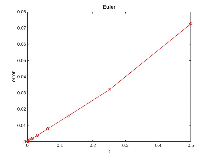
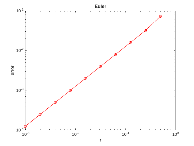
We can see that for Euler $p\approx 1$.

Runge

error = zeros(no_approx,1);
for ei=1:no_approx
  x = solve(@runge, @logistic, 0, 2, x0, h(ei), timepoint);
  error(ei) = norm(exact-x);
end
[p,q]=regrese(h,error);

figure;
plot(h,error,'-ro');
title('Runge');
xlabel('\tau');
ylabel('error');

figure;
loglog(h,error,'-ro');
title('Runge')
xlabel('\tau');
ylabel('error');
fprintf('Runge = %f + %f x log10(tau)\n', q, p);

Runge = -0.806076 + 2.124211 x log10(tau)

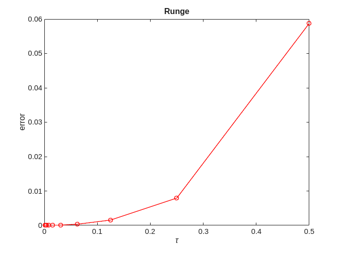
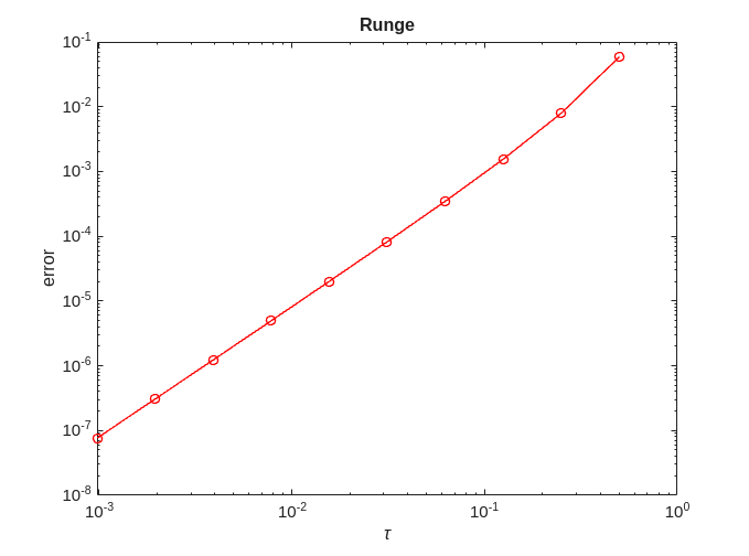
We can see that for Runge $p\approx 2$.

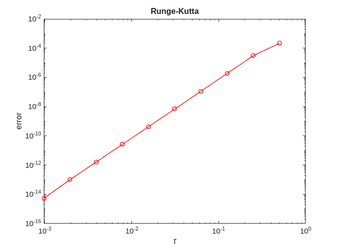
Runge-Kutta

error = zeros(no_approx,1);
for ei=1:no_approx
  x = solve(@rk_classical, @logistic, 0, 2, x0, h(ei), timepoint);
  error(ei) = norm(exact-x);
end
[p,q]=regrese(h,error);

figure;
plot(h,error,'-ro');
title('Runge-Kutta');
xlabel('\tau');
ylabel('error');

figure;
loglog(h,error,'-ro');
title('Runge-Kutta')
xlabel('\tau');
ylabel('error');
fprintf('Runge-Kutta = %f + %f x log10(tau)\n', q, p);

Runge-Kutta = -2.228915 + 3.970831 x log10(tau)

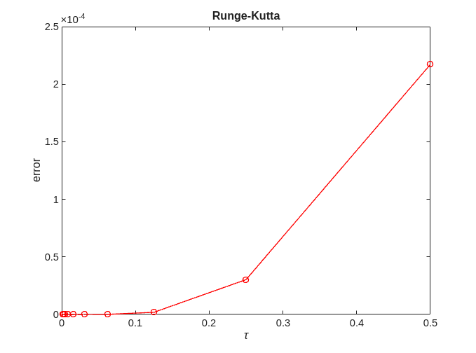
We can see that for Runge-Kutta $p\approx 4$.

Heun

error = zeros(no_approx,1);
for ei=1:no_approx
  x = solve(@heun, @logistic, 0, 2, x0, h(ei), timepoint);
  error(ei) = norm(exact-x);
end
[p,q]=regrese(h,error);

figure;
plot(h,error,'-ro');
title('Heun');
xlabel('\tau');
ylabel('error');

figure;
loglog(h,error,'-ro');
title('Heun')
xlabel('\tau');
ylabel('error');
fprintf('Heun = %f + %f x log10(tau)\n', q, p);

Heun = -1.068869 + 2.057883 x log10(tau)

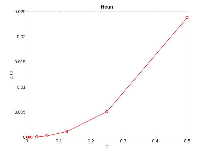
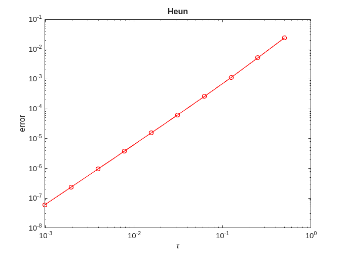
We can see that for Heun $p\approx 2$.

Implicit Euler

Note, we start from h=1/4, as Implicit Euler fails to converge for h=1/2

for tol=[0.1,0.001,0.0001,0.00001]
  error = zeros(no_approx,1);
  h = 0.5.^(1+(1:no_approx))'; % start from 1/4 (.5^2)
  for ei=1:no_approx
    x = solve(@ieuler, @logistic, 0, 2, x0, h(ei), timepoint, tol);
    error(ei) = norm(exact-x);
  end
  [p,q]=regrese(h,error);

  figure;
  plot(h,error,'-ro');
  title(['Implicit Euler (tol=' num2str(tol) ')']);
  xlabel('\tau');
  ylabel('error');

  figure;
  loglog(h,error,'-ro');
  title(['Implicit Euler (tol=' num2str(tol) ')']);
  xlabel('\tau');
  ylabel('error');
  fprintf('Implicit Euler (tol=%f) = %f + %f x log10(tau)\n', tol, q, p);
end

Implicit Euler (tol=0.100000) = -0.818021 + 1.027462 x log10(tau)
Implicit Euler (tol=0.001000) = -0.902095 + 0.998404 x log10(tau)
Implicit Euler (tol=0.000100) = -0.901978 + 0.998643 x log10(tau)
Implicit Euler (tol=0.000010) = -0.901963 + 0.998655 x log10(tau)

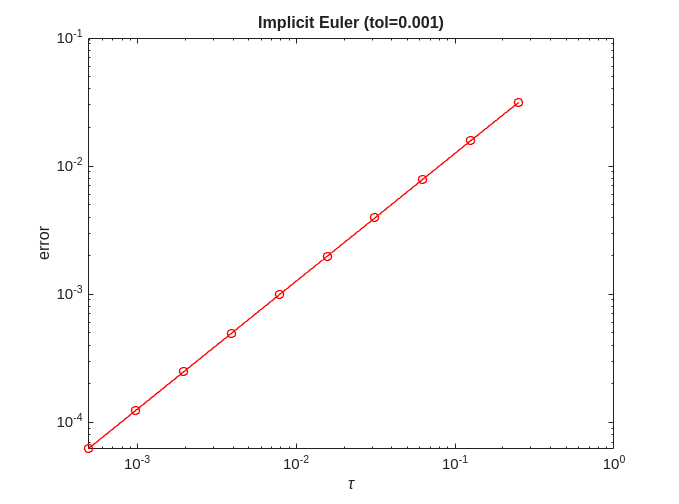
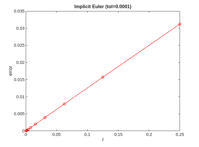
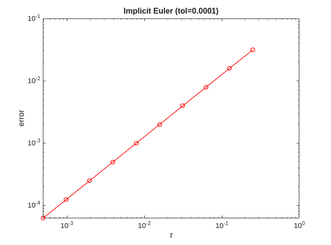
We can see that for Implicit Euler $p\approx 1$.

Crank-Nicholson

for tol=[0.1,0.001,0.0001,0.00001]
  error = zeros(no_approx,1);
  for ei=1:no_approx
    x = solve(@crank_nicholson, @logistic, 0, 2, x0, h(ei), timepoint, tol);
    error(ei) = norm(exact-x);
  end
  [p,q]=regrese(h,error);

  figure;
  plot(h,error,'-ro');
  title(['Crank-Nicholson (tol=' num2str(tol) ')']);
  xlabel('\tau');
  ylabel('error');

  figure;
  loglog(h,error,'-ro');
  title(['Crank-Nicholson (tol=' num2str(tol) ')']);
  xlabel('\tau');
  ylabel('error');
  fprintf('Crank-Nicholson (tol=%f) = %f + %f x log10(tau)\n', tol, q, p);
end

Crank-Nicholson (tol=0.100000) = -1.985822 + 1.712550 x log10(tau)
Crank-Nicholson (tol=0.001000) = -0.985795 + 2.277137 x log10(tau)
Crank-Nicholson (tol=0.000100) = -1.254186 + 2.037598 x log10(tau)
Crank-Nicholson (tol=0.000010) = -1.305834 + 2.001045 x log10(tau)

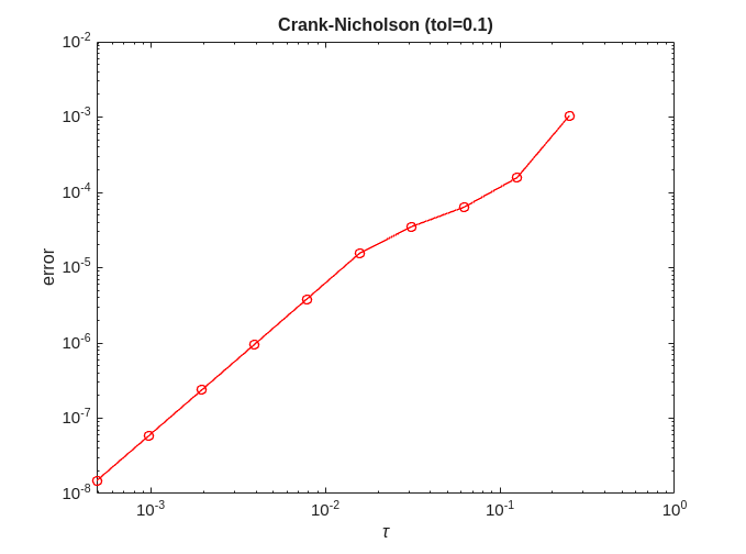
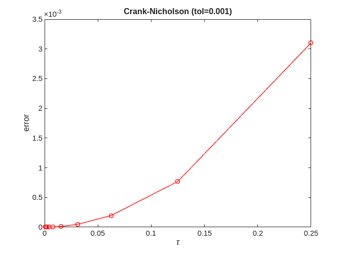
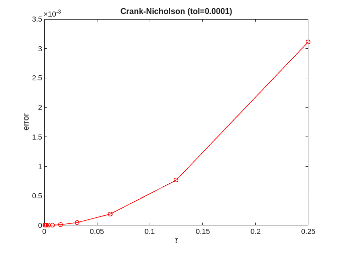
We can see that for Crank-Nicholson $p\approx 2$ providing tol is sufficiently small

Solve function

Function to run the specified solver and extract the value at the specified timepoint

function y = solve(solver, field, t0, T, x0, h, timepoint, varargin)
%SOLVE Use the specified ODE solver to solve the ODE and get value at
%  specified time point
%
% Parameters:
%  solver    -- ODE solve to use
%  field     -- Right hand side function of ODE system: x'=f(t,x)
%  t0        -- Initial time
%  T         -- End time (T > t0)
%  x0        -- Initial value
%  h         -- Size of time step (h <= T-t0)
%  timepoint -- Timepoint to get numerical solution at
%  varargin  -- Extra arguments to pass to the solver
%
% Returns: Computed value at timepoint

[t,x] = feval(solver, field, t0, T, x0, h, varargin{:});

n1 = floor((timepoint-t0)/h);
n2 = ceil((timepoint-t0)/h);

if n1 == n2
    y = x(n1+1,:);
else
    y1 = x(n1+1,:);
    y2 = x(n2+1,:);
    t1 = t(n1+1);
    t2 = t(n2+1);
    y = y1 + (y2-y1)*(timepoint-t1)/(t2-t1);
end

end

Linear Regression

Function to perform linear regression in log-log coordinates

function [p,q]=regrese(x,y)
% REGRESE Compute linear regression
%
% Fits the line log10(y) = p log10(x) + q  in "loglog" coordinates
%
% Returns: p, q
%          p = estimated order of the method

data=[log10(x),log10(y)];
m=length(x);

A=[data(:,1), ones(m,1)];
coeffs=A\data(:,2);
p=coeffs(1);
q=coeffs(2);
end

end

Published with MATLAB® R2025b