Contents

Question 1

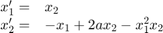
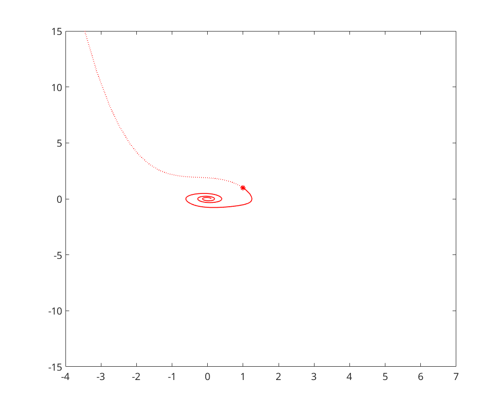
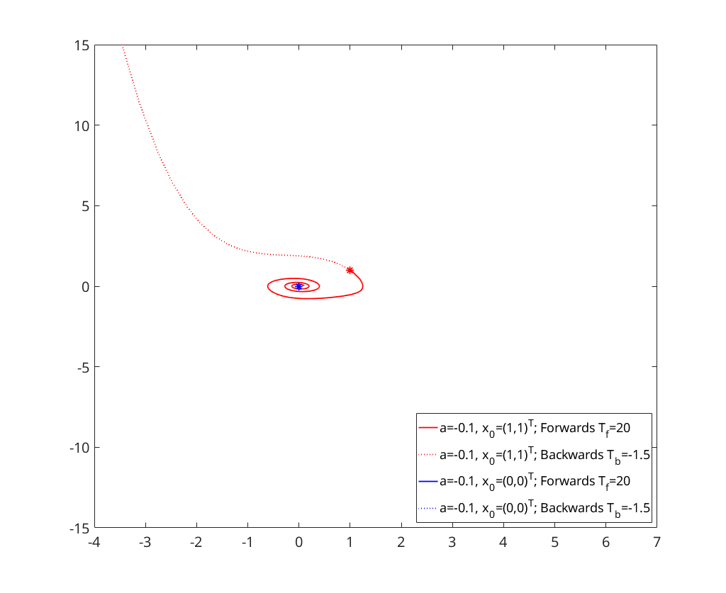
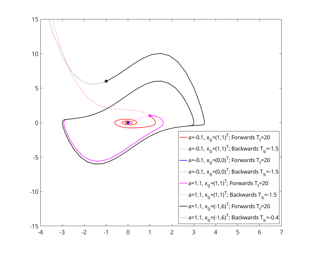
We consider Van der Pol's oscillator:

$\begin{array}{rl} x_1'=& x_2 \\ x_2'=& -x_1+2ax_2-x_1^2x_2 \end{array}$

function q1_solution

a) Backwards & Forwards solve with ode23s

$a=-0.1$; Initial condition $x_0=(1,1)^T$

a = -0.1;
x0 = [1;1];
% Plot initial point
plot(x0(1),x0(2),'r*','HandleVisibility','off');
hold on;
xlim([-4 7]);
ylim([-15, 15]);
% Solve forward
[~,x]=ode23s(@(t,x)vdpol(t,x,a), [0,20], x0);
plot(x(:,1),x(:,2),'r','DisplayName','a=-0.1, x_0=(1,1)^T; Forwards T_f=20');
% Solve backward
[~,x]=ode23s(@(t,x)vdpol(t,x,a), [0,-1.8], x0);
plot(x(:,1),x(:,2),':r','DisplayName','a=-0.1, x_0=(1,1)^T; Backwards T_b=-1.5');

$a=-0.1$; Initial condition $x_0=(0,0)^T$

a = -0.1;
x0 = [0;0];
% Plot initial point
plot(x0(1),x0(2),'b*','HandleVisibility','off');
hold on;
legend('Location','SouthEast');
% Solve forward
[~,x]=ode23s(@(t,x)vdpol(t,x,a), [0,20], x0);
plot(x(:,1),x(:,2),'b','DisplayName','a=-0.1, x_0=(0,0)^T; Forwards T_f=20');
% Solve backward
[~,x]=ode23s(@(t,x)vdpol(t,x,a), [0,-1.5], x0);
plot(x(:,1),x(:,2),':b','DisplayName','a=-0.1, x_0=(0,0)^T; Backwards T_b=-1.5');

$a=1.1$; Initial condition $x_0=(1,1)^T$

a = 1.1;
x0 = [1;1];
% Plot initial point
plot(x0(1),x0(2),'m*','HandleVisibility','off');
hold on;
% Solve forward
[~,x]=ode23s(@(t,x)vdpol(t,x,a), [0,20], x0);
plot(x(:,1),x(:,2),'m','DisplayName','a=1.1, x_0=(1,1)^T; Forwards T_f=20');
% Solve backward
[~,x]=ode23s(@(t,x)vdpol(t,x,a), [0,-1.5], x0);
plot(x(:,1),x(:,2),':m','DisplayName','a=1.1, x_0=(1,1)^T; Backwards T_b=-1.5');

$a=1.1$; Initial condition $x_0=(-1,6)^T$

a = 1.1;
x0 = [-1;6];
% Plot initial point
plot(x0(1),x0(2),'k*','HandleVisibility','off');
hold on;
% Solve forward
[~,x]=ode23s(@(t,x)vdpol(t,x,a), [0,20], x0);
plot(x(:,1),x(:,2),'k','DisplayName','a=1.1, x_0=(-1,6)^T; Forwards T_f=20');
% Solve backward
[~,x]=ode23s(@(t,x)vdpol(t,x,a), [0,-0.4], x0);
plot(x(:,1),x(:,2),':k','DisplayName','a=1.1, x_0=(-1,6)^T; Backwards T_b=-0.4');

b) Analysis of Steady States

We now study the steady state $x^*=(0,0)^T \in R^2$ for $a=-1.1,0.5,1.1$

disp('----------------------------------------');
vdpol_steady(-1.1);
disp('----------------------------------------');
vdpol_steady(0.5);
disp('----------------------------------------');
vdpol_steady(1.1);
disp('----------------------------------------');

----------------------------------------
a = -1.100000

Jacobian:
                   0   1.000000000000000
  -1.000000000000000  -2.200000000000000

Eigenvalues:
  -0.641742430504416
  -1.558257569495584

Maximum of real part of eigenvalues: -0.641742

Steady state is A-stable
----------------------------------------
a = 0.500000

Jacobian:
     0     1
    -1     1

Eigenvalues:
  0.500000000000000 + 0.866025403784438i
  0.500000000000000 - 0.866025403784438i

Maximum of real part of eigenvalues: 0.500000

Steady state is NOT A-stable
----------------------------------------
a = 1.100000

Jacobian:
                   0   1.000000000000000
  -1.000000000000000   2.200000000000000

Eigenvalues:
   0.641742430504416
   1.558257569495584

Maximum of real part of eigenvalues: 1.558258

Steady state is NOT A-stable
----------------------------------------

c) Numerical approximation

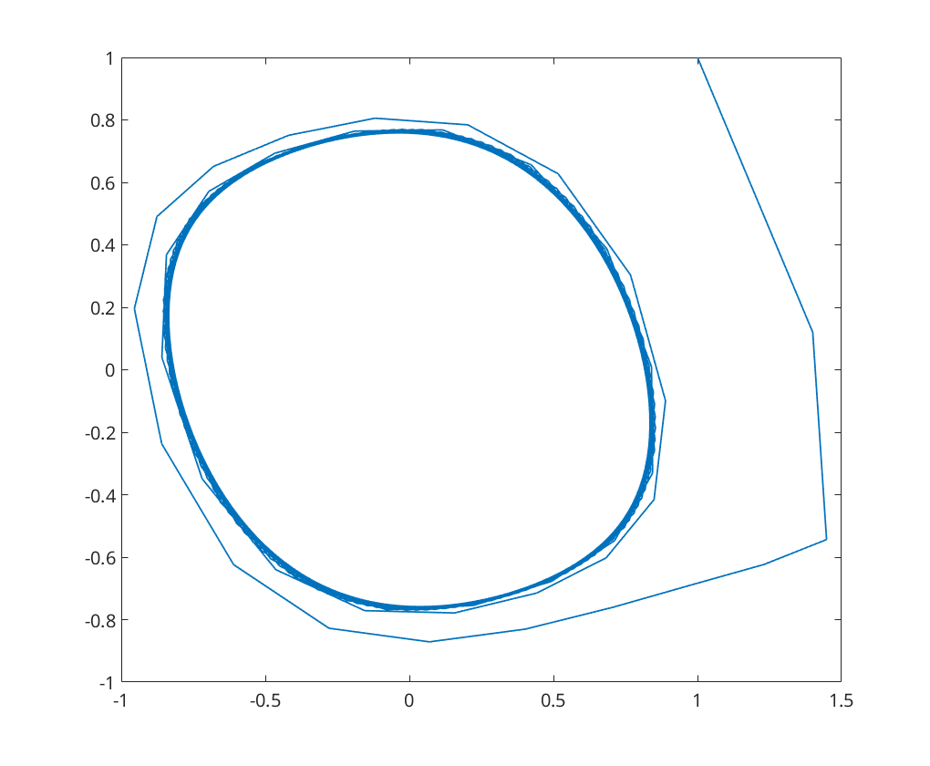
We calculate the numerical approximation for initial condition $x_0=(1,1)^T$ and $a=-0.1$

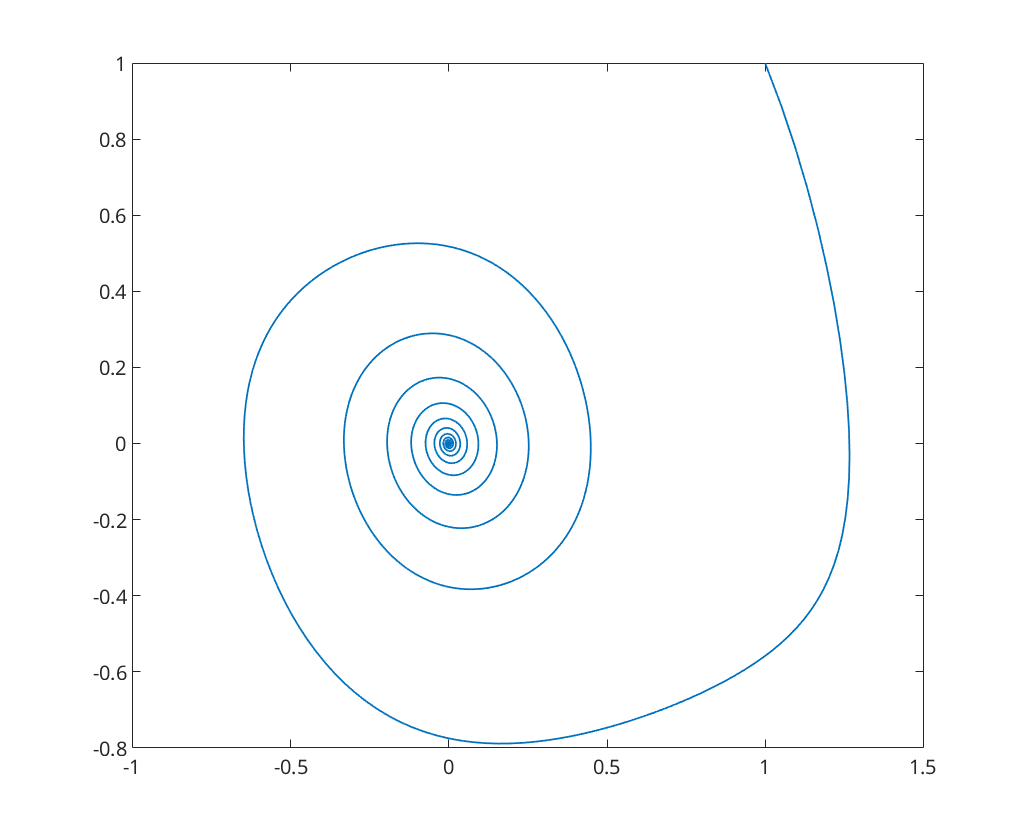
We start using Euler with $\tau = 0.4$ and notice that the solution does not converge to the steady state, instead getting stuck in an orbit around the steady state as the the fixed point of the Euler method with $\tau=0.5$ is NOT $A$-stable

figure;
a = -0.1;
x0 = [1;1];
[~,x]=eul(@(t,x)vdpol(t,x,a), 0, 120, x0, 0.4);
plot(x(:,1),x(:,2));

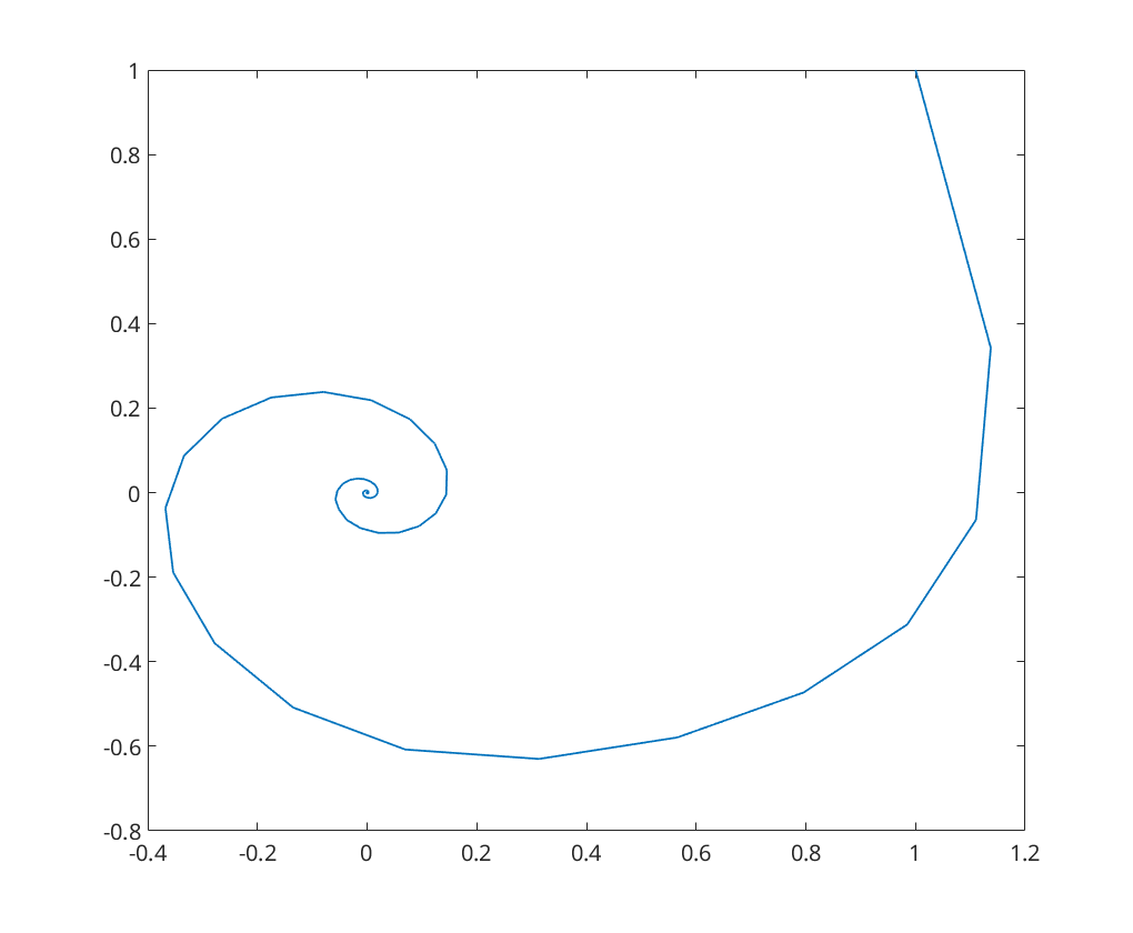
Decreasing the time step size to $\tau=0.05$ the fixed point is now $A$-stable

figure;
a = -0.1;
x0 = [1;1];
[~,x]=eul(@(t,x)vdpol(t,x,a), 0, 120, x0, 0.05);
plot(x(:,1),x(:,2));

For implicit Euler, the fixed point is $A$-stable even with $\tau = 0.4$

figure;
a = -0.1;
x0 = [1;1];
[~,x]=ieuler(@(t,x)vdpol(t,x,a), 0, 120, x0, 0.4);
plot(x(:,1),x(:,2));

Utility function for analysis of Steady State $x^*=(0,0)^T \in R^2$

function vdpol_steady(a)

fprintf('a = %f\n\n', a);

% Jacobian at steady state:
A = [0 1; -1 2*a];
disp('Jacobian:');
disp(A);

% Eigenvalues:
ev = eig(A);
disp('Eigenvalues:');
disp(ev);

% A-stable?:
fprintf('Maximum of real part of eigenvalues: %f\n\n', max(real(ev)));

if max(real(ev)) < 0
    disp('Steady state is A-stable')
else
    disp('Steady state is NOT A-stable')
end
end

end

Published with MATLAB® R2023a