Octave: Newton's and 2nd order method
%graphics_toolkit('gnuplot');
%% number of grid points / time step
N=50;
h=1/N;
%% initial condition / exact (explicit) solution
x0=1;
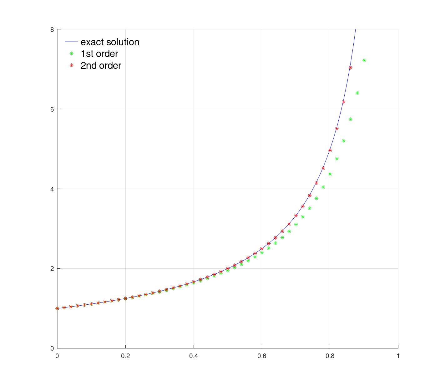
ex = @(t) x0 ./ (1 - x0.*t);
clf; figure(1,'position',[1000,300,900,800]), hold on
axis([ 0 1 0 8 ]), grid on;
%% plot the exact solution (in blue)
dt = 0.01;
I = 0:dt:1;
plot(I,ex(I),'-b');
%%% Newton's method
Xnewton = zeros(1,N);
Xnewton(1) = x0;
for i = 1:(N-1)
Xnewton(i+1) = Xnewton(i) + h*(Xnewton(i))^2;
end
T = h*(0:N-1);
%%% plot the points (green stars)
plot(T,Xnewton,'*g');
%plot(T,Xnewton,'..k');
%pause
%%% 2nd order method
Xsecond = zeros(1,N);
Xsecond(1) = x0;
for i = 1:(N-1)
Xsecond(i+1) = Xsecond(i) + h*(Xsecond(i))^2 + h^2*(Xsecond(i))^3;
end
%%% plot as red stars
plot(T,Xsecond,'*r');
%plot(T,Xsecond,'-k');
%title( sprintf('h=%f',h) );
%%% display legend
h = legend( "exact solution","1st order","2nd order" );
legend( h , "location", "northwest");
legend( h , "boxoff") ;
set (h, "fontsize", 15);
%%% optionally, save the pictures as pdf/png
%print -dpdf "demo1.pdf"
%print -dpng "demo1.png"
%print -djpg "obr3.jpg"
%%% wait for a key ....
pause;